A QoS-configurable failure detection service for internet applications

Abstract

Unreliable failure detectors are a basic building block of reliable distributed systems. Failure detectors are used to monitor processes of any application and provide process state information. This work presents an Internet Failure Detector Service (IFDS) for processes running in the Internet on multiple autonomous systems. The failure detection service is adaptive, and can be easily integrated into applications that require configurable QoS guarantees. The service is based on monitors which are capable of providing global process state information through a SNMP MIB. Monitors at different networks communicate across the Internet using Web Services. The system was implemented and evaluated for monitored processes running both on single LAN and on PlanetLab. Experimental results are presented, showing the performance of the detector, in particular the advantages of using the self-tuning strategies to address the requirements of multiple concurrent applications running on a dynamic environment.

1 Introduction

Consensus [1] and other equivalent problems, such as atomic broadcast and group membership are used to implement dependable distributed systems [2, 3]. However, given the FLP impossibility [4], i.e., consensus can not be solved deterministically in asynchronous distributed systems in which even a single process can fail by crashing, deploying high-available distributed systems on the Internet is a challenge. In order to circumvent the impossibility of solving consensus in asynchronous distributed systems, Chandra and Toueg introduced failure detectors based on timeouts [5–7].

Failure detectors are used to monitor processes of any application running on a network. Failure detectors provide process state information. In this way, failure detectors are described as distributed “oracles” that supply information about the state of processes. Each application that needs process state information accesses the failure detector as a local module. Failure detectors can make mistakes, i.e., report that a fault-free process has failed or vice-versa and, therefore are said to be unreliable. It is impossible to implement a failure detector that always provides the precise information, e.g. consider that a monitored process that is correct suddenly crashes; until the crash is perceived, the failure detector will report that the monitored process is correct. Chen, Toueg and Aguilera [8] defined a set of criteria to evaluate the quality of the service (QoS) of failure detectors. The authors defined a set of metrics to quantify the speed (e.g. how fast a process crash is detected) as well as the accuracy (e.g. how well it avoids mistakes) of failure detectors.

In this work we describe an Internet Failure Detection Service (IFDS) that can be used by applications that consist of processes running on independent autonomous systems of the Internet. IFDS reconfigures itself to provide the QoS level required by the applications. Chen et al. [8] and Bertier et al. [9] have investigated how to configure QoS parameters according to the network performance and the application needs. The parameters include the upper bounds on the detection time and mistake duration, and the lower bound on the average mistake recurrence time. Bertier et al. extended that approach by computing a dynamic safety margin which is used to compute the timeout. The main contribution of the present work is that IFDS handles multiple concurrent applications, each with different QoS requirements. In this way, two or more applications with different QoS requirements can use the detector to monitor their processes, and IFDS reconfigures itself so that all requirements are satisfied.

IFDS was implemented using SNMP (Simple Network Management Protocol) [10]. Processes of a distributed application access the failure detector through a SNMP interface. In the proposed service, monitors execute on each LAN where processes are monitored. The monitor is implemented as a SNMP agent that keeps state information of both local and remote processes. The implementation of the service is based on a SNMP MIB (Management Information Base) called fdMIB (failure detector MIB), which can be easily integrated to distributed applications. The implementation also employs Web Services [11] that enable the transparent communication between processes running on different Autonomous Systems (AS). As Web Services are used as gateways for SNMP entities, they are transparent to the applications. Experimental results are presented for distributed applications with monitored processes executing both on a single LAN and in the PlanetLab [12], the worldwide research testbed. Results include an evaluation of the overhead incurred by the failure detector as the QoS parameters vary, the failure detection time, and average mistake rate.

The rest of the paper is organized as follows. Section 2 is a short introduction to failure detector and also presents an overview of related work. In Section 3 IFSD is specified, in particular we describe how the service dynamically adapts to network conditions and multiple concurrent application requirements. The architecture of the proposed failure detector service is described in Section 4. The implementation and experimental results are described in Sections 5 and 6, respectively. Section 7 concludes the work.

2 Failure detectors and related work

Consensus is a basic building block of fault-tolerant distributed computing [3, 13]. Informally, processes execute a consensus algorithm when they need to agree on a given value, which depends on an initial set of proposed values. The problem can be easily solved if the system is synchronous, i.e., there are known bounds on the time it takes to communicate messages and on how fast (or slow) processes execute tasks. On the other hand, if those time limits are unknown, i.e., the system is asynchronous, and processes can fail by crashing, then consensus becomes impossible to solve. This is a well-known result proved by Fischer, Lynch, and Paterson in 1985 and also known as the FLP impossibility [4]. Note that this impossibility assumes the most “benign” type of fault, the crash fault, in which one process simply stops to produce any output given any input.

As consensus is such an important problem and time limits for sending messages and executing tasks in real systems, such as the Internet, are unknown, the FLP impossibility represents a challenge for developing practical fault-tolerant distributed systems. Furthermore, it has been proved that several other important problems are equivalent to consensus so that they are also impossible to solve under the same assumptions. These include atomic broadcast, leader election, and group membership, among others [14].

Unreliable failure detectors were proposed by Chandra and Toueg [5] as an abstraction that, depending on its properties, can be used to solve consensus in asynchronous systems with crash faults. In this sense, a failure detector is a distributed oracle that can be accessed by a process to obtain information about the state of the other processes of the distributed system. Each process accesses a local module implementing the failure detector, which basically outputs a list of processes suspected of having failed. In a broad sense failure detectors can be used to monitor processes of any application running on a network. Furthermore, the failure detector must have a well-known interface through which it provides process state information.

The root of the FLP impossibility is that it is difficult to determine in an asynchronous system whether a process has crashed or is only slow. This problem also affects failure detectors: in asynchronous systems they can make mistakes. For example, fault-free but slow processes can be erroneously added to the list of failed processes. Thus, failure detectors are said to be unreliable, and instead of indicating which processes have failed, they indicate which processes are suspected to have failed. Chandra and Toueg in [5] give a classification of unreliable failure detectors in terms of two properties: completeness and accuracy. Completeness characterizes the ability of the failure detector to suspect faulty processes, while accuracy restricts the mistakes that the detector can make. Completeness is said to be strong if every process that crashes is permanently suspected by all correct processes. Otherwise, if at least one correct process suspects every process that has crashed, then completeness is weak. Accuracy is classified as strong if no process is suspected before it crashes, and weak if some correct process is never suspected. Both completeness and accuracy are eventual if they only hold after a finite but unknown time interval.

The most common approach to implement failure detectors is to employ heartbeat messages, which are sent periodically by every monitored process. Based on the observed message arrival pattern, the failure detector computes a timeout interval. If a heartbeat message is not received within this timeout interval, the monitored process is suspected to have crashed. A key decision to implement failure detectors is the choice of algorithm to compute a precise timeout interval. If the timeout interval is too short, crashes are quickly detected, but the likeliness of wrong suspicions is higher. Conversely, if the timeout interval is too long, wrong suspicions will be rare, but this comes at the expense of long detection times [15]. An adaptive failure detector can automatically update the timeout intervals and for this reason it is generally chosen to implement failure detectors on real networks [16].

In [8], Chen, Toueg, and Aguilera specify criteria to evaluate quality of service (QoS) provided by failure detectors. They define a set of metrics that quantify both the failure detector speed (how fast crashes are detected) and accuracy (how well it avoids mistakes). Three basic metrics (see Fig. 1) are defined as described below.

• Detection time ( T _D ): represents the time interval from the instant process p has crashed to the instant at which the failure detector starts to suspect p permanently.

  Fig. 1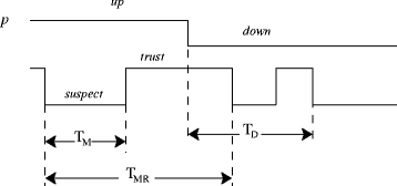

  

  Basic metrics that represent the QoS of a failure detector

• Mistake recurrence time ( T _MR ): this metric corresponds to the time interval between two consecutive mistakes, i.e., it represents how frequently the failure detector makes mistakes.

• Mistake duration ( T _M ): represents the time it takes for the failure detector to correct a mistake.

Other metrics are derived from those above; such as the Query accuracy probability ( P _A ) which corresponds to the probability that the output of the failure detector is correct at a random instant of time. Besides defining the above metrics, Chen et al. also propose a failure detector algorithm that adapts itself according to how metrics are configured and the characteristics of the network on which it is running, including the message loss probability (p _L ), the expected message delay (E(D)) and message delay variance (V(D)).

Bertier et al. [9] extend the approach proposed by Chen et al. by implementing a failure detector in two layers: an adaption layer runs on top of a traditional heartbeat-based failure detector. The adaptation layer configures the Quality of Service (QoS) of the failure detector according to application needs. The purpose is also to minimize both network and processor overhead. While Chen’s failure detector computes the timeout interval based on the expected arrival time of the next message, Berthier’s also uses a safety margin which is continuously updated according to Jacobson’s TCP (Transmission Control Protocol) timeout algorithm.

Another work that extends the original approach of Chen et al. was [17] proposed by Dixit and Casimiro. The authors define an alternative way to configure the QoS parameters, which is based on the stochastic properties of the underlying system. Initially, the user must provide a specification of the average mistake recurrence time (T _MR defined above) and the minimum coverage (C ^L), which corresponds to a lower bound on the probability that heartbeat messages are received before the timeout interval expires. These parameters are used by a configurator which relies on another system called Adaptare that is a middleware that computes the timeout by estimating distributions based on the stochastic properties of the system on which the failure detector is running. The system was evaluated and presented sound results, especially in terms of the average mistake recurrence time and coverage.

In [16], Bondavalli and Falai present an extensive comparison of a large number of failure detectors executed on a wide area network. They conclude that no failure detector presents at the same time high speed and high accuracy. In particular, they show that using a more accurate predictor to compute the timeout interval does not necessarily imply on better QoS. The authors conclude that a perfect solution for the failure detection problem does not exist.

Tomsic et al. [18] introduced a failure detection algorithm that provides QoS and adapts to sudden changes in unstable network scenarios. The failure detector is called Two Windows Failure Detector (2W-FD) and it uses two sliding windows: a small window (to react rapidly to changes in network conditions) and a larger window (to make better estimations when the network conditions change gradually). The authors show that their algorithm presents better QoS when compared to others running on networks under unstable conditions.

In [19] the authors design an autonomic failure detector that is capable of self-configuration in order to provide the required QoS. In [20] a failure detector that is capable of self-configuration is applied to a cloud computing environment.

Network monitoring systems based on the Internet Simple Network Management Protocol (SNMP) have been used to feed system information to failure detectors. Lima and Macedo in [21] explore artificial neural networks in order to implement failure detectors that dynamically adapt themselves to communication load conditions. The training patterns used to feed the neural network were obtained from a network monitoring system based on SNMP.

Wiesmann, Urban, and Défago present in [22] the SNMP-FD framework, a SNMP-based failure detector service that can be executed on a single LAN. Several MIBs are defined to keep information such as identifiers of hosts running monitors, identifiers and state of each monitored process, heartbeat intervals, heartbeat counters, among others.

In [23], a failure detector service for Internet-based distributed systems that span multiple autonomous systems (AS) is proposed. The service is based on monitors which are capable of providing global process state information through a SNMP interface. The system is based both on SNMP and Web services, which allow the communication of processes across multiple AS’s.

To the best of our knowledge, the present work is the first that proposes a SNMP-based failure detector service with self-configurable Quality of Service. Given the requirements of multiple simultaneous applications, we present two strategies that allow the detector to self-configure. With respect to previous SNMP-based implementations of failure detectors, the major benefit of our proposed service is that it allows the user to specify QoS requirements for each application that is monitored, including: the failure detection time, mistake recurrence time and mistake duration. Given this input, and the perceived network conditions, our service configures and continuously adapt the failure detector parameters, including the heartbeat rate. Furthermore, as mentioned above, the proposed service can take into consideration the QoS requirements for multiple simultaneous applications to configure the system. Other SNMP-based implementations of failure detectors do not support QoS parameters to be input to the system, thus the user must manually configure the system and, worse, keep reconfiguring the system manually as network conditions and requirements change. Furthermore, IFDS introduces a novel implementation strategy in which SNMP objects themselves execute process monitoring – other works employ a separate daemon for that purpose.

3 IFDS: failure detection and QoS configuration

In this section, IFDS is described and specified. Initially, the system model is presented. Next, we give details on how IFDS computes adaptive timeout intervals, and then describe the configuration of IFDS parameters which are based both on network conditions and on applications QoS requirements. Besides showing how parameters are configured to monitor a single application process, two strategies are proposed to configure IFDS when multiple processes are monitored with different QoS requirements. The first strategy is called η _max and it maximizes monitoring parameters to encompass the needs of all processes; the second strategy is called η _GCD and it computes the greatest common divisor of the corresponding parameters.

3.1 System model

We assume a distributed system S={p ₁,p ₂,…,p _n ,} that consists of n units that are called processes but also correspond to hosts. The system is asynchronous but augmented with the proposed failure detector, i.e. we assume a partially synchronous system. Processes communicate by sending and receiving messages. Every pair of processes is connected by a communication channel, i.e. the system can be represented by a complete graph. Processes fail by crashing, i.e., by prematurely halting. Every process in S has access to IFDS as a local failure detector module. IFDS returns process state information: correct or suspected. Monitored processes periodically send heartbeat messages. Timeouts are used to estimate whether processes have crashed.

3.2 IFDS adaptive timeout computation

Arguably, the most important feature of a failure detector is how precisely the timeout interval is computed. Remember that if a message is expected from a monitored process and it does not arrive before the timeout interval expires, then the process is suspected to have failed. A timeout interval that is too long increases the failure detection time, and a timeout interval that is too short increases the number of mistakes, i.e., correct processes can be frequently suspected to have crashed. Given the Internet characteristics in time and space, as well as different applications requirements, it is impossible to employ constant, predefined timeouts. Practical failure detectors must employ dynamic timeouts that are adaptive in the sense that they are reconfigured according to changing network conditions and application requirements.

IFDS computes the timeout interval (τ) for the next expected message using information about the arrival times of recently received messages. Note that for a given monitored host, multiple processes running on that host can be monitored, each with different QoS requirements. A single message is periodically expected from the host conveying information about the status of all its processes. IFDS computes the timeout with a strategy inspired on the works of Chen et al. [8] and Bertier et al. [9]. Chen’s failure detector allows the configuration of QoS parameters according to network performance and the application needs. Bertier et al. extend that approach by also considering a dynamic safety margin to compute the timeout.

Chen et al. [8] compute an estimation of the arrival time (EA) of the next message based on the arrival times of previously received messages. That estimation plus a constant safety margin (α) are the basis for calculating the next timeout. Bertier et al. extend that approach by dynamically estimating α (the safety margin) using Jacobson’s TCP timeout algorithm [24]. EA is computed as the weighted average of the n last message arrival intervals, where n is the window size for keeping historical records.

IFDS thus computes the timeout interval (τ) for monitoring a process based on an estimation of the next heartbeat arrival time (EA) plus a dynamic safety margin (α). Let’s consider two processes: p and q, p monitors q. Every η time units, q sends a heartbeat to p. Let m ₁,m ₂,…,m _k be the k most recent heartbeat messages received by p. Let T _i be the time interval that each heartbeat took to be received by p, i.e. the time interval that elapsed since heartbeat i−1 had been received until heartbeat i is received, measured with the local clock. EA can be estimated as follows:

$$ \begin{aligned} EA_{k+1} = \frac{1}{k} \left(\sum_{i=1}^{k} T_{i} - \eta\right) + (k+1)\eta \end{aligned} $$

(1)

EA _k+1 is the expected time instant at which the next message (the k+1- th message) will arrive. The next timeout will expire at:

$$ \begin{aligned} \tau_{(k+1)} = EA_{(k+1)} + \alpha_{(k+1)} \end{aligned} $$

(2)

The safety margin α is computed based on Jacobson’s TCP algorithm and is used to correct the error of the estimation for the arrival of the next message. Let A _i be the arrival time of heartbeat i, error _(k) represent the error of the k-th message computed as follows:

$$ \begin{aligned} error_{(k)} = A_{k} - EA_{k} - delay_{(k)} \end{aligned} $$

(3)

In the expression (4), delay _(k+1) is the estimated delay of next message which is computed in terms of the error _(k). γ represents the weight of the new measure, Jacobson suggests γ=0.1:

$$ \begin{aligned} delay_{(k+1)} = delay_{(k)} + \gamma.error_{(k)} \end{aligned} $$

(4)

var _(k+1) represents the error variation, and it computed from first iteration; initially var _(k) is set to zero.

$$ \begin{aligned} var_{(k+1)} = var_{(k)} + \gamma.(|error_{(k)} - delay_{(k+1)}|) \end{aligned} $$

(5)

The safety margin α _(k+1) is then computed as shown below, where β and ϕ are constant weights for which we used β=1,ϕ=4 and γ=0.1.

$$ \begin{aligned} \alpha_{(k+1)} = \beta.delay_{(k+1)} + \phi.var_{(k+1)} \end{aligned} $$

(6)

The timeout interval τ is thus adjusted after each heartbeat message arrives.

3.3 Configurig the failure detector service based on QoS parameters

In this subsection, we initially describe how IFDS is configured based on the QoS requirements of a single application. Then the strategy is extended to handle multiple concurrent applications, each with different QoS requirements. Notice that even if two applications use the detector to monitor the same process, they may still have different QoS requirements. In this case, based on the different QoS requirements, a single heartbeat interval is chosen to monitor the process, i.e., the one that satisfies all requirements. On the other hand, the detection time used by the service for each application may be different. For example, one application may need a short detection time while the other can cope with a larger interval. If the heartbeat message is delayed and arrives after the shorter detection time but before the larger detection time, only the first application is informed that a false suspicion occurred.

As shown in Fig. 2, the detector receives as input from an application the following parameters:

• ${T_{D}^{U}}$: an upper bound on the detection time;

  Fig. 2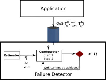

  

  Finding η. IFDS receives the QoS parameters from an application

• ${T_{M}^{U}}$: an upper bound on the average mistake duration;

• $T_{MR}^{L}$: a lower bound on the average mistake recurrence time

Thereafter, the failure detector processes the input data and seeks a suitable value for η, as shown next.

3.3.1 QoS configuration for a single application

In Fig. 2, IFDS receives the QoS parameters from an application. The part of the Failure Detector devoted to the configuration of QoS parameter consists of two modules: Estimator and Configurator. Given the messages (heartbeats) received from a monitored process, the Estimator computes three parameters: the message loss probability (p _L ), the message delay variance (V(D)), and the estimation for the arrival time of the next message (EA). The message loss probability is computed as p _L =L/k where k is the total number of messages that have been sent and L is the number of messages that were lost. V(D) is computed from the observations of the message arrival times.

The configurator module runs Algorithm 1 adapted from [8, 9] to compute η, i.e., the heartbeat interval to be used by a monitored process in order to keep the quality of service required by the application. Algorithm 1 is described next.

Algorithm 1 consists of two steps. The main purpose of Step1 is to compute an upper bound for the heartbeat interval η _max , given the input values provided by the application: the upper bound on the detection time (${T_{D}^{U}}$), upper bound on the average mistake duration (${T_{M}^{U}}$), and lower bound on the average mistake recurrence time ($T_{MR}^{L}$). First, θ is computed (line 12) which reflects the failure detection probability, based on both the probability that a message is received (1−p _L ), the message delay variance (V(D)), and the required detection time (${T_{D}^{U}}$). Now remember that η _max must be chosen to meet the required upper bounds on the detection time and mistake duration time. Thus η _max is set to the minimum of the upper bound of the detection time (${T_{D}^{U}}$) or the detection probability times the upper bound of the mistake duration rate ($\theta *{T_{M}^{U}}$).

Note that if either θ=0 or ${T_{D}^{U}}=0$ or ${T_{M}^{U}}=0$ then the maximum heartbeat interval is zero; this means that there is no heartbeat interval that is able to guarantee the QoS requirements. In this case, Step 2 is not executed.

The main purpose of Step 2 of the algorithm is to find the smallest η that respects the third QoS parameter: $T_{MR}^{L}$, the mistake recurrence time. Step2 computes η as follows. η is initially equal to η _max . Then η is reduced by 1 % at each iteration until f(η)geq $T_{MR}^{L}$. This reduction factor (1 %) was chosen experimentally as it gives precise results, close to $T_{MR}^{L}$ – if we use 10 % the precision is lost we can get a value that is acceptable but too distant from $T_{MR}^{L}$. As proved in [8], for each value of η,f(η) computes the probability that the required mistake recurrence time ($T_{MR}^{L}$) is satisfied. Note that if η decreases f(η) increases, the opposite is also true. For this reason, we always reduce the value of η until $f({\eta }) \geq T_{MR}^{L}$. When this condition holds, the largest η that satisfies $T_{MR}^{L}$ has been computed.

Next we give an example of the computation of η by Algorithm 1.

An application (App ₁) specifies the following QoS requirements: ${T_{D}^{U}}=$ 30 s (i.e., a crash failure is detected within 30 s), ${T_{M}^{U}}=$ 60 s (i.e., the failure detector corrects its mistakes within 60 s), and $T_{MR}^{L}=$ 432000s (i.e., the failure detector makes at most one mistake each 5 days). Furthermore, the message loss probability is p _L = 0.0 and the delay variance is V(D)= 0.01. The algorithm in Step1 computes γ= 0.99 and η _max =min(30, 59.99). In Step2, the input values are processed initializing η equal to 30.00. After that, the algorithm continuously reduces the value of η until f(η)≥ 432, 000. The final value is η= 14.6 s, which is employed by monitored processes to periodically send heartbeat messages to meet the QoS requirements of App ₁.

Actually, the final value of η found in Step2 is the largest interval that satisfies the QoS requirements. Thus, a shorter interval, 0 <η≤ 14.6, can also be used for the example.

3.3.2 QoS configuration for multiple applications

When several applications are monitoring multiple processes with IFDS, each can have different QoS requirements. IFDS computes a heartbeat interval (η) for the monitored processes that simultaneously satisfies the QoS requirements of all applications. In order to understand why this can save monitoring messages consider a simple example in which 100 hosts connected on a single LAN each of which executes 100 processes that are be monitored. To make the example as simple as possible assume that all processes employ the same heartbeat interval. If one uses a separate FD service to monitor each process than 10,000 heartbeat messages are sent per interval. Using our shared/simultaneous monitoring strategy this number reduces to only 100 messages, each host employs one heartbeat message for all its processes.

In this work we assume that the different processes can need different heartbeat intervals to satisfy their QoS requirements. In order to determine a common heartbeat interval to be used by all processes, two different approaches are proposed: η _max and η _GCD , described below.

The η _max approach to adapt η to all application requests computes $\eta _{max} = min \left (\gamma {{T_{M}^{U}}}_{1}, {{T_{D}^{U}}}_{1}, \gamma {{T_{M}^{U}}}_{2}, {{T_{D}^{U}}}_{2}, \ldots, \gamma {{T_{M}^{U}}}_{n},{{T_{D}^{U}}}_{n}\right)$, where $i=1\ldots n, {{T_{M}^{U}}}_{i}$ and ${{T_{D}^{U}}}_{i}$ are the QoS requirements of application i. Algorithm 1 can be then used after this modification is introduced.

The other proposed approach is called η _GCD and in this case we compute the GCD (Greatest Common Divisor) among all η _i ,i=1…m, m is the number of QoS requirements. The idea is that if a process sends heartbeats every x units of time, and if x divides y, it also sends heartbeats every y units of time. Each η _i is first transformed to a new η i′ as follows: η i′ = 2ⁿ so that 2ⁿ<η _i and $\eta _{i}' \in \mathbb {Z}^{+}$. The final η _GCD =GCD(η i′,…,η n′). Note that η _GCD must be > 0, otherwise it is impossible to apply this approach.

Note that η _max gives the largest possible heartbeat interval that satisfieds the QoS requirements. Thus in order to have a safety margin it is recommended to use an interval shorter than that, such as given by η gcd. η _GCD is always smaller than η _max for a given system. For this reason, using the η _GCD approach produces a larger number of messages on the network than η _max . On the other hand, it has advantages such as a reduction of the failure detection time (T _D ) and improvement of the query accuracy probability (P _A ).

Consider an extension of the example given above for one application (App ₁) where a second application (App ₂) runs on the same host as App ₁. App ₂ QoS requirements are as follows: ${T_{D}^{U}}=$ 15 s (i.e., a crash failure is detected within 15 seconds), ${T_{M}^{U}}=$ 30 s (i.e., the failure detector corrects its mistakes within 30 seconds) and $T_{MR}^{L}=$ 864000 s (i.e., the failure detector makes at most one mistake each 10 days). We assume that the message loss probability is p _L = 0.0 and the delay variance is V(D)= 0.01. First consider the η _max approach. In Step1 of the algorithm η _max =min((30,59.99)app ₁,(29.99,15.00)app ₂)=15.00. In Step2, the final value is computed as η=7.2 s, then the algorithm uses this value to ensure the QoS parameters for both applications (App ₁ and App ₂).

On the other hand, if we use the η _GCD approach we have: App ₁: η ₁= 14.6 →η1′=8; App ₂: η ₂= 7.2 →η2′= 4; η _GCD =GCD(4,8)→ 4. Thus, η _GCD = 4 s. As mentioned above, we can notice that η _GCD is smaller than η _max .

Our implementation is capable of self-adapting to QoS violations caused by network conditions. If IFDS detects that the network cannot sustain the minimum QoS requirements, it readjusts η by increasing its value. For instance, in the example above, η can be readjusted to another value as long as it complies with the following condition: η≤ 14.6. Hence, Algorithm 1 is used to find a value of η that satisfies QoS requirements of as many applications as possible under the current network conditions.

4 IFDS: architecture

In this section we describe the architecture of the proposed Internet failure detection service. Figure 3 shows IFDS monitoring processes on two LAN’s: A and B. These two LANs are geographically distributed and connected through the Internet. The number of monitored networks can be greater than two. For each network, there is both a Monitor Host and Monitored Hosts. As the names denote, a Monitored Host runs the processes that are monitored. The Monitor Host runs applications that are responsible for monitoring processes. Applications and other Monitors can subscribe to receive state information about specific processes.

Fig. 3

IFDS architecture

Initially, every application that needs to obtain information about the states of monitored processes configures the quality of service (QoS) it expects from IFDS. Then, the detection service computes the heartbeat interval (η) that must be applied in order to provide the required QoS. The Monitor Host then configures η on every Monitored Host, so that periodically at an η interval, the monitored host will send back a heartbeat message to the Monitor Host.

As we shall see in Section 5, SNMP (Simple Network Management Protocol) is used by the Monitor and Monitored Hosts to exchange messages on a LAN. Each Monitored Host is registered on a SNMP MIB (Management Information Base). If the Monitor and Monitored hosts are located on different networks and must communicate across the Internet, they employ Web Services. In this case, a SNMP message is encapsulated with and transmitted using SOAP (Simple Object Access Protocol).

Note that all monitoring is done locally on each domain. Monitors on different domains communicate to obtain process state information. This communication is implemented in two ways. Either the local Monitor queries the remote Monitor to obtain process state information, or, alternatively, the Monitor can register at a remote monitor to receive notifications whenever the state of remote monitored processes changes. In this case, a SNMP message is encapsulated with and transmitted using SOAP (Simple Object Access Protocol).

Web Services are thus used as a gateway for entities that implement SNMP to communicate remotely across the Internet. The use of Web Services is transparent to the user application, which employs only SNMP as the interface to access the failure detector. There are situations in which Web Services are not involved, i.e., when all the communication occurs on a local LAN. When a Monitor issues a query to another monitor running remotely, a virtual connection is open (using Web Services), and a remote procedure is executed that provides the required information.

When an application needs to communicate with a Monitor running remotely, it has an option to do that directly using Web Services. For example, consider the system in Fig. 3, suppose that the application process (App ₁) on Network A needs to learn information about the status of a process running on Network B. In this case, App ₁ invokes the corresponding Web Services that in turn executes the SNMP operation on Network B.

When the Monitor Host detects that the state of a monitored process on the same LAN has changed, it updates the corresponding entry and sends the new state information to all applications and other Monitors that have subscribed to receive information about that particular process.

All information about the state of processes is stored in a MIB called fdMIB (failure detector MIB). In Section 5 we present detailed information about this MIB and its implementation.

5 IFDS: implementation

As mentioned in the previous section, IFDS was implemented with SNMP and Web Services. SNMP is used by the Monitor and Monitored Hosts to exchange messages and each Monitored Host must be registered on the fdMIB, shown in Fig. 4. fdMIB consists of three groups: the Monitor Host Group, Monitored Host Group, and Application Notify Group. These three object groups are described below. Note that we propose a single MIB that maintains information about all IFDS modules.

Fig. 4

fdMIB objects. In this figure we propose a single MIB that maintains information about all IFDS modules

The Application Notify Group ( appNotifyGroup ) keeps information about QoS parameters. Each application that is supposed to receive state information about a process must give the following parameters to fdMIB: the upper bound on the detection time (TD_U), the mistake duration time (TM_U), and the lower bound on the average mistake recurrence time (TMR_L). These parameters are described in Section 3. We also described how IFDS computes the heartbeat interval η, given the application parameters.

Another object of the appNotifyGroup is receiveHB (see Fig. 4) which is used to receive heartbeat messages from a monitored process. Every time a heartbeat message arrives, fdMIB updates the corresponding process state object in the monitorHostGroup table.

In order to receive notifications, an application subscribes at the Monitor Host to receive SNMP traps (notifyTrap) with process state information. The application will be notified whenever the Monitor detects a change of the state of the monitored process. Object statusChange is also updated to store 0, if the monitored process is correct, and 1 otherwise. Note that besides receiving traps (alarms) the application can at any time check the state of any monitored process by querying the corresponding MIB object.

The Monitor Host Group (monitorHostGroup) stores information about monitored processes, including IP addresses (ipAddr), port numbers (portNumber), process IDs (processID), state (statusHost), number of false detections (falseDetection), heartbeat interval required (reqFreq), an estimation of the probabilistic behavior of message delays (V_D), message loss probability (P_L), QoS parameters (current_TD, current_TM and current_TMR) these parameters are continuously updated and are used to check whether any QoS requirement has been broken (e.g., current_TD >TD_U), among others. Objects of the monitorHostGroup trigger and execute process monitoring. For instance, they can start threads that receive heartbeat messages and compute timeouts.

The Monitored Host Group ( monitoredHostGroup ) is responsible for sending heartbeat messages. It is executed on a host that is monitored. In order to communicate with the Monitor, the following objects are maintained: Monitor IP address (ipMonitor), Monitor port (portMonitor), monitored process OID (myOidInMonitor, an Object Identifier is a name used to identify the monitored process in the MIB), heartbeat interval (frequencyHB), and the process identifier in the local host (processID).

6 IFDS: experimental results

In this section we report results of several experiments executed in order to evaluate the proposed failure detection service. Experiments were conducted on both an Ethernet LAN and PlanetLab [12]. Three independent applications were used each with different QoS requirements, as shown in Table 1. All applications run on the same host. For instance, App ₁ requires that the time to detect failures to be at most 8 seconds, i.e., ${T_{D}^{U}}$ = 8 s. On average the failure detector corrects its mistakes within one minute, i.e., ${T_{M}^{U}}$ = 60 s. Finally, the failure detector makes at most one mistake per month, i.e., $T_{MR}^{L}$ = 30 days (2592000000 in ms). In the experiments, we assumed p _L = 0.01 and V(D) = 0.02, the sliding window (W) size is defined individually for each experiment.

Table 1 QoS requirements

IFDS configuration can be simply done using the regular snmpset command; for instance the command below is executed to configure the monitorHostGroup table with the required QoS parameters (Fig. 4). In this example, App ₁ monitors a process on a host with IP address 192.168.1.1, the port is 80, and the QoS parameters are those shown in Table 1.

snmpset -v1 -c private localhost.1.3.6.1.4.1.18722.1. 2.1.1.2.1 s 192.168.1.1:8:80:60:2592000000

The snmpset command shown above is used to update the value of a SNMP object. This command uses the following parameters: host address on which the MIB is deployed (localhost), the id of the object to be updated (.1.3.6.1.4.1.18722.1.2.1.1.2.1) and the data that is to be written on the object (192.168.1.1:8:80:60:2592000000).

Using Algorithm 1 (presented in Section 3.3) to compute the heartbeat interval for the three applications shown in Table 1, we get η _max = min(1.954467, 3.901890, 4.694764). Thus, in this case the value of η is 1.954467 (enough to meet the QoS requirements of all three applications). If instead we use the η _GCD strategy on the same data in Table 1, we get GCD=min(1,2,4). Thus η=1 again enough to monitor App ₁,App ₂, and App ₃.

6.1 Experimental results: LAN

The LAN experiments were executed on two hosts: the monitor host was based on an Intel Core i5 2.50 GHz processor, with 4 GB of RAM, running Linux Ubuntu 12.04 with kernel 3.2.0-58; the monitored host was an Intel Core i5 CPU 3.20 GHz, with 4 GB RAM running Linux Ubuntu 13.10 with kernel 3.2.0-58. The hosts were on a 100 Mbps Ethernet LAN. The fdMIB was implemented using Net-SNMP version 5.4.4.

The first experiment was executed to evaluate how IFDS adapts to changes in the heartbeat frequency. How does the failure detector react and reconfigures itself? Figure 5 shows the expected arrival time (EA curve) and timeout (Timeout curve) computed by IFDS as the monitored host sends 200 heartbeat messages to the monitor host. The figure also shows the measured RTT (RTT curve). From the beginning to the 50th heartbeat message the interval between two messages (the Heartbeat Freq curve) is 1 s. Then from the 51st message to the 150th message this interval grows to 5 s, after that the frequency reduces to 1 s again.

Fig. 5

Adapting the timeout for different heartbeat intervals

The Figure shows that initially (first 10 messages) the timeout takes a while to stabilize. Then when the heartbeat frequency changes from 1 to 5 s, the EA and timeout curves show that after a short while IFDS could clearly adapt the timeout interval to the new heartbeat frequency. During that short while (after the 50th message) the Timeout curve remains below the Heartbeat Freq curve: during this time IFDS incurs in false suspicions. After a couple of messages the timeout grows enough to correct the mistakes. The Figure also shows how IFDS reacts when the heartbeat frequency reduces back to 1 second (from the 150th message). The EA and Timeout curves show that after a few messages IFDS readapts itself to the new situation.

Next we show – for the same experiment – both the QoS requirements (given by the application), as well as the current value of the QoS parameters computed by IFDS from the actual monitoring. The objective of this experiment is to show that the applications’ QoS requirements are not violated. Figure 6 a and b show the QoS parameters for the same experiment described in Fig. 5. Besides the EA, Heartbeat Freq and RTT curves that also appeared in Fig. 5, these Figures also show the detection time (TD curve), the mistake duration time (TM curve), the detection times required by the applications: App1 TDU, App2 TDU, and App3 TDU curves.

Fig. 6

Global QoS is not violated. Subfigure (a) shows the T _D and T _M performance, and in subfigure (b) describes the T _MR performance

In Fig. 6 a we can observe 6 false detections (TM curve), notice that the QoS requirements (Table 1) are never violated. In the same Figure, the detection time T _D is always less than App1 TDU, App2 TDU and App3 TDU. This means that the false suspicions shown in Fig. 6 a remain transparent to the applications, i.e. they are not noticed by any of the applications, even when the heartbeat frequency grows to 5 s. Note that after message 50 the TD curve gets very close to but does not grow above App1 TDU.

A similar situation can be seen in Fig. 6 b, in which the mistake recurrence rate is checked. Note that the lower limit of the T _MR QoS parameter required by the applications is 30 days (Table 1). Curve TMR shows the average T _MR taking into account the false suspicions that occurred (TM curve). If we compute the average for the whole time the experiment was executed, it is 13, 086 ms, which is below the required value for this QoS metric. However, the real IFDS T _MR does not take into account the false suspicions that are not reported to the applications. As discussed, none of the false suspicions was ever reported to the applications, thus there was no mistake and mistake recurrence time and there is no QoS violation.

Next we describe an experiment designed to compare the two strategies proposed for monitoring multiple processes simultaneously: η _max and η _GCD . The experiment duration time was 60 min. The results for this experiment are shown in Table 2. This table shows: the heartbeat interval η (in seconds), the detection time T _D , the mistake duration time T _M , and the mistake recurrence time T _MR , the P _A metric (described below) plus the number of heartbeat messages sent during the experiment, and the number of false detections. During the experiment we simulated two false suspicions by omitting heartbeat messages. The P _A metric corresponds to the probability that the application will make a query about a given monitored process and that the reply is correct, in the sense that it reflects the real state of the monitored process. This metric was described in Section 2 and can be computed as follows:

$$ \begin{aligned} P_{A} = 1-\frac{E(T_{M})}{E(T_{MR})} \end{aligned} $$

(7)

Table 2 Comparing the two strategies: η _max and GCD

The results in Table 2 show that the heartbeat interval computed by η _max is 1.95 s, while for η _GCD it is equal to 1 s. The next results are a consequence of these intervals. Remember that a higher heartbeat interval means that less messages are sent, and thus the overhead of η _max (1754 messages) is lower than the overhead of η _GCD (3551 messages). On the hand, the opposite happens to the detection time T _D : as η _GCD ’s heartbeat interval is shorter, its detection time T _D is also shorter (1.32 s) while for η _max it grows to 2.46 s. The same happens to the mistake duration time (T _M ) and P _A : the shorter the heartbeat interval, the shorter the mistake duration and the higher the probability that IFDS replies the correct state. Although the time recurrence time (T _MR ) also reduces for a shorter heartbeat interval, the variation is lower than for the other parameters.

A discussion on these results leads to the conclusion that there is a trade-off. While η _max proves is the best strategy for applications that do not require a small detection time (which is the case for instance for monitoring remote processes via the Internet) η _GCD presents a shorter detection time and the best results for the P _A metric. This strategy is thus the better suited to monitor processes on a single LAN, where the applications generally do not tolerate long delays.

Next we evaluate the amount of resources required by IFDS. Figure 7 shows CPU and memory usage. We gradually increased the number of monitored objects. For each measure 10 samples were collected and the service was run for 60 min. The experiment comprises both the registration of each object in the fdMIB (which corresponds to setting the information about monitored processes such as IP address and port) and the transmission of heartbeat messages. A very short heartbeat interval of 1 millisecond was chosen to stress the system. As shown in Fig. 7 a, memory usage grows linearly but remains low: it never reaches 0.2 %. In Fig. 7 b we can see that up to 100 objects, there is a consistent increase in CPU usage. After that (100 objects), although peak values do increase, the average CPU usage remains stable around 7 %. CPU usage can be considered low enough. For example, the SNMP-based implementation of a failure detector by Wiesmann, Urban and Defago [22] reaches up to 11 % CPU utilization for 1 millisecond heartbeat interval.

Fig. 7

Evaluating the performance as the number of monitored objects increases. Subfigure (a) shows the Memory Usage, and in subfigure (b) shows the CPU Usage

6.2 Experimental results: PlanetLab

The last experiment was executed to investigate the time overhead of using Web Services for communicating across the Internet. In particular we were interested in comparing the time to report an event using a pure SNMP solution with one that also uses Web Services. We executed IFDS to monitor processes running on PlanetLab nodes located in the five continents: South America (Brazil), North America (Canada), Europe (Italy), Asia (Russia) and Oceania (New Zealand). PlanetLab hosts exchange information in two ways: using SNMP and Web Services. The time was computed using a monitor and a monitored process running in Brazil. After the monitor detects a failure it notifies yet another monitor. Then, we measured the time interval from the instant a fault was injected up to the instant the second monitor is notified. In other words, the time to report an event is the sum of the detection time plus the time to notify the event. In Fig. 8, we compare the time using SNMP only and Web services. As expected, WS takes longer to report an event: on average of 14.44 % more than SNMP, which we consider an acceptable overhead.

Fig. 8

Time to notify a failure using SNMP and WS

From the results in Fig. 8 it is also possible to see that the notification time respects the physical distance between hosts. The process that is the closest to the monitor (running on the Brazilian host) presents a notification time of approximately 1.31 s. As the physical distance between hosts increases, the notification time also increases, reaching up to approximately 2.01 s for the monitored process that runs on the New Zealand host. From these observations one can conclude that an application may take location also into account in order to determine the level of QoS that can be obtainable from each process – for example, the detection time of a process that is close by will be certainly lower than that of a process that is on another continent.

7 Conclusion

In this paper, we described the architecture and implementation of the Internet Failure Detection Service (IFDS). IFDS configures itself to meet the QoS requirements of multiple simultaneous applications as well as network conditions. Two strategies (η _max and η _GCD ) were proposed to compute the interval (η) on which monitored processes send heartbeats. IFDS was implemented using SNMP and Web Services for enabling communication among applications across the Internet. Experimental results were presented, in which the failure detector service ran both on a single LAN and on PlanetLab. In this case, monitored processes run on hosts of five continents. The results show the effectiveness of the adaptive timeout with different intervals of heartbeat messages. On the one hand, the η _max strategy is more suitable for monitoring remote processes where applications can tolerate longer delays. On the other hand, the η _GCD strategy is better suited for monitoring processes running on a LAN.

Future work includes developing reliable distributed applications on top of the proposed IFDS, including State Machine Replication, as well an atomic broadcast service, both of which also rely on consensus. Making the link between an FD that provides QoS and consensus is certainly a relevant topic for future research. How can the QoS parameters have an influence on the execution of a consensus algorithm? How to specify the required QoS levels, taking into account features of the consensus algorithm as well as multiple process features – including location, for instance.

References

Turek J, Shasha D. The Many Faces of Consensus in Distributed Systems.IEEE Comput. 1992; 25(6):8–17.
Guerraoui R, Rodrigues L. Introduction to Reliable Distributed Programming. Berlin: Springer; 2006.
Charron-Bost B, Pedone F, Schiper A, (eds).Replication: Theory and Practice. Berlin: Springer; 2010.
Fischer MJ, Lynch NA, Paterson MS. Impossibility of distributed consensus with one faulty process. J ACM. 1985; 32(2):374–82.
Chandra TD, Toueg S. Unreliable failure detectors for reliable distributed systems. J ACM. 1996; 43(2):225–67.
Freiling FC, Guerraoui R, Kuznetsov P. The failure detector abstraction. ACM Comput Surv. 2011; 43(2):1–40.
Delporte-Gallet C, Fauconnier H, Raynal M. Fair synchronization in the presence of process crashes and its weakest failure detector. In: 33rd IEEE International Symposium on Reliable Distributed Systems (SRDS’14). Japan: IEEE Computer Society, Nara: 2014.
Chen W, Toueg S, Aguilera MK. On the quality of service of failure detectors. In: International Conference on Dependable Systems and Networks (DSN’00). New York: IEEE Computer Society: 2000.
Bertier M, Marin O, Sens P. Performance analysis of a hierarchical failure detector. In: International Conference on Dependable Systems and Networks (DSN’03). San Francisco, USA: IEEE Computer Society: 2003.
Harrington D, Presuhn R, Wijnen B. An Architecture for Describing Simple Network Management Protocol (SNMP) Management Frameworks. In: Request for Comments 3411 (RFC3411). United States: RFC Editor: 2002.
Christensen E, Curbera F, Meredith G, Weerawarana S. Web Services Description Language(WSDL) Version 1.1.http://www.w3.org/TR/wsdl. Access Feb 2016.
An open platform for developing, deploying, and accessing planetaryscale services. http://www.planet-lab.org/. Access May 2015.
Turek J, Shasha D. The many faces of consensus in distributed systems. IEEE Comput. 1992; 25(6):8–17.
Cachin C, Guerraoui R, Rodrigues L. Introduction to Reliable and Secure Distributed Programming 2nd edn.Berlin: Springer; 2011.
Hayashibara N, Defago X, Katayama T. Two-ways adaptive failure detection with the ϕ-failure detector. In: International Workshop on Adaptive Distributed Systems. Italy: Sorrento: 2003.
Falai L, Bondavalli A. Experimental evaluation of the qos of failure detectors on wide area network. In: International Conference on Dependable Systems and Networks (DSN’05). Yokohama: IEEE Computer Society: 2005.
Dixit M, Casimiro A. Adaptare-fd: A dependability-oriented adaptive failure detector. In: 29th IEEE Symposium on Reliable Distributed Systems (SRDS’10). Delhi: IEEE Symposium: 2010.
Tomsic A, Sens P, Garcia J, Arantes L, Sopena J. 2w-fd: A failure detector algorithm with qos. In: IEEE International Parallel and Distributed Processing Symposium (IPDPS’15). Washington: IEEE Computer Society: 2015.
de Sá AS, de Araújo Macêdo RJ. Qos self-configuring failure detectors for distributed systems. In: Distributed Applications and Interoperable Systems (DAIS) 2010. Amsterdam, The Netherlands: Springer Berlin Heidelberg: 2010.
Xiong N, Vasilakos AV, Wu J, Yang YR, Rindos AJ, ZHOU Y, Song WZ, Pan Y. A self-tuning failure detection scheme for cloud computing service. In: The 26th IEEE International Parallel & Distributed Processing Symposium (IPDPS) 2012. Shanghai: IEEE Computer Society: 2012.
Lima F, Macêdo R. Adapting failure detectors to communication network load fluctuations using snmp and artificial neural nets. In: Dependable Computing, Second Latin-American Symposium (LADC’05). Salvador: Springer Berlin Heidelberg: 2005.
Wiesmann M, Urbán P, Défago X. An SNMP based failure detection service. In: 25th IEEE Symposium on Reliable Distributed Systems (SRDS’06). Leeds: IEEE Computer Society: 2006.
Moraes DM, Duarte Jr EP. A failure detection service for internet-based multi-as distributed systems. In: 17th IEEE International Conference on Parallel and Distributed Systems (ICPADS’11). Tainan: IEEE Computer Society: 2011.
Jacobson V. Congestion avoidance and control. In: Symposium Proceedings on Communications Architectures and Protocols (SIGCOMM’88). USA: ACM, Stanford: 1988.
Acknowledgements
This work was partially supported by grants 309143/2012-8 and 141714/2014-0 from the Brazilian Research Agency (CNPq).
Authors’ contributions
RCT carried out the implementation and ran the experiments; together with the other authors he also participated in writing this paper. EPD Jr. supervised the definition of the proposed architecture, supervised the implementation and experiments, and wrote the paper. PS and LA proposed the strategies for monitoring multiple processes that represents the main scientific contribution of this paper, they revised the architecture as it was proposed and also revised the written paper. All authors read and approved the final manuscript.
Competing interests
We confirm that I have read SpringerOpen’s guidance on competing interests and have included a statement indicating that none of the authors have any competing interests in the manuscript.
Author information
Authors and Affiliations
Corresponding author
Rights and permissions
Open Access This article is distributed under the terms of the Creative Commons Attribution 4.0 International License(http://creativecommons.org/licenses/by/4.0/), which permits unrestricted use, distribution, and reproduction in any medium, provided you give appropriate credit to the original author(s) and the source, provide a link to the Creative Commons license, and indicate if changes were made.
About this article
Cite this article
Turchetti, R.C., Duarte, E.P., Arantes, L. et al. A QoS-configurable failure detection service for internet applications. J Internet Serv Appl 7, 9 (2016). https://doi.org/10.1186/s13174-016-0051-y
Received:
Accepted:
Published:
DOI: https://doi.org/10.1186/s13174-016-0051-y