DG2CEP: a near real-time on-line algorithm for detecting spatial clusters large data streams through complex event processing

Abstract

Spatial concentrations (or spatial clusters) of moving objects, such as vehicles and humans, is a mobility pattern that is relevant to many applications. Fast detection of this pattern and its evolution, e.g., if the cluster is shrinking or growing, is useful in numerous scenarios, such as detecting the formation of traffic jams or detecting a fast dispersion of people in a music concert. On-Line detection of this pattern is a challenging task because it requires algorithms that are capable of continuously and efficiently processing the high volume of position updates in a timely manner. Currently, the majority of approaches for spatial cluster detection operate in batch mode, where moving objects location updates are recorded during time periods of a certain length and then batch-processed by an external routine, thus delaying the result of the cluster detection until the end of the time period. Further, they extensively use spatial data structures and operators, which can be troublesome to maintain or parallelize in on-line scenarios. To address these issues, in this paper we propose DG2CEP, a parallel algorithm that combines the well-known density-based clustering algorithm DBSCAN with the data stream processing paradigm Complex Event Processing (CEP) to achieve continuous and timely detection of spatial clusters. Our experiments with real-world data streams indicate that DG2CEP is able to detect the formation and dispersion of clusters with small latency while having higher similarity to DBSCAN than batch-based approaches.

1 Introduction

This paper investigates the possibility and limitations of an on-line and near real-time (few seconds) detection of spatial clusters from large position data streams generated by moving objects (e.g., humans, vehicles, drones). Spatial clusters [1] are concentrations of moving objects in some region, for example, a massive street protest, a music concert, a traffic jam, etc. A fast detection of this pattern and its evolution, e.g., if the cluster is shrinking or growing, is useful in numerous scenarios, such as detecting the formation of traffic jams, detecting a fast dispersion of people in a music concert and optimizing urban traffic [2–5].

However, implementing timely spatial cluster detection from large position data streams poses several challenges [6, 7]. First, it has to employ efficient algorithms and data structures to cope with the high arrival rate of the position data (location updates) stream and intrinsic complexity of mutually comparing the location of all moving objects. Second, it must be able to detect arbitrary clusters shapes, for example, a traffic jam that reaches over several neighborhoods or a human crowd that spans across the seashore of a city. Third, it has to provide timely results that reflect the current clustering scenario to enable a fast reaction by decision makers. Finally, it must be able to track its evolution, for example, providing a continuous view of how clusters are growing or merging.

To address these issues, the majority of data stream clustering algorithms [8–11] operate in an on/off-line batch framework [6, 12], where position data is first accumulated during a given time period (on-line phase) and they are processed in batch by a specific cluster detection function (off-line phase). The main problem with this approach is that this function only processes the data items within each batch separately and defers the cluster detection process until the end of the off-line phase. Thus, since it delivers results only at discrete points of time it is complicated to provide fresh results and a continuous view of the clusters’ evolution. Further, due to the batch nature, it can happen that temporally and spatially close location updates end up in different batches, possibly preventing a cluster to be detected.

Motivated by such limitations, this paper investigates means of achieving on-line (continuously) and rapidly (near real-time) detection of spatial clusters from large position data streams. This problem has the following three sub-questions:

• 1 How similar is the on-line and near real-time clustering result to the ground-truth result, i.e., the one obtained using the traditional DBSCAN’s [13] off-line clustering algorithm?

• 2 How scalable is this approach w.r.t. the data stream volume, i.e., is it possible to provide or maintain the clustering quality when increasing the throughput of the data stream?

• 3 Finally, can this approach continuously monitor, in near real-time, the spatial cluster’s evolution?

To address such questions, this paper proposes DG2CEP (Density-Grid Clustering using Complex Event Processing), a grid-based (counting) algorithm that combines the traditional density-based clustering algorithm DBSCAN [13] with the data stream processing paradigm Complex Event Processing (CEP) [14, 15]. One of the main ideas in DG2CEP is to change the problem semantic from distance computations (between the moving objects location) to counting. To do this, we subdivide the spatial domain into a grid, an efficient index data structure for spatial data. Then, rather than measuring the distance between each pair of moving objects, we count the number of objects mapped to each cell. Cells that contain more than a given threshold of moving objects are further analyzed. This process triggers an expansion step that recursively merges a dense cell with its adjacent neighbor. Since cells are aligned in a grid, the expansion step is straightforward.

With this method, the main performance bottleneck is no longer the distance comparison between moving objects, but the number of grid cells. This entire approach is described using the CEP data stream processing paradigm. CEP provides a set of real-time data stream analytics and pattern primitives [16, 17] through continuous queries, such as filter, join, and sequence.

This paper is based on the thesis results described in [18], which revisit, combines and extend the preliminary ideas discussed in [19] and [20]. The first paper only describes the initial CEP algorithm required to detect spatial cluster while the latter described an heuristic to address collateral effects caused by the grid-like approach. Here, we present a holistic approach that further develops and combine these two parts to provide a complete and efficient on-line algorithm. For instance, we extended the CEP algorithm rules to accommodate the heuristic logic to improve algorithm precision. We also present an extensive performance analysis and in-depth discussions about the advantages and limitations of the heuristic-enhanced DG2CEP when compared to the original DG2CEP, to the original density-based algorithm, DBSCAN [13], and to the batch-based D-STREAM [21].

The main and novel contributions of this paper are:

• An on-line counting algorithm based on grid-density clustering, designed as a network of CEP continuous query and pattern primitives, that is able to continuously and timely detect (near real-time) spatial clusters and its evolution from large position data streams.

• A counting heuristic that mitigates the collateral effects of the answer loss (blind spot) problem [22, 23] that appears due to the usage of a grid structure to index and cluster spatial data.

• A scalable event processing network architecture that can process data in parallel and be distributed to process higher data stream throughputs.

This paper is organized as follows. Section 2 briefly restate the paper problem and present the fundamental topics used to address it. After that, Section 3 presents the main related-works. Section 4 presents the proposed algorithm, DG2CEP, while Section 5 presents a counting heuristic that mitigates the collateral effects of transforming the problem from distance comparison to counting. Section 6 presents the evaluation experiment used to validate the proposed algorithm. Finally, Section 7 presents the concluding remarks and limitations of our approach. It also points to future works that can address or explore these issues.

2 Fundamental concepts

2.1 Spatial clustering

Spatial clustering is the process of identifying agglomerations in spatial data [24], such as those produced by moving objects (e.g., vehicles and pedestrians). To exemplify this concept, consider the spatial data of vehicles (moving objects) in Fig. 1. This figure illustrates three moving object clusters. Each cluster contains at least five moving objects, which need to be close and connected to one another. Note that moving objects that are not close to other objects are considered noise.

Fig. 1

Spatial clustering of moving objects in an urban scenario

The Density-Based Spatial Clustering of Applications with Noise (DBSCAN) [13] is a classic algorithm that uses density thresholds to discover such clusters. We decided to base our approach in this algorithm due to its ability to discover arbitrary cluster shapes, e.g., a cluster represented by a complex polygon such as a traffic jam that spans several different streets.

DBSCAN searches for concentrations of spatial data points, in our case, moving objects’ current position. To do that, it uses two density parameters, an ε radius and the minimum density minPts of spatial points, to specify the density-based cluster definition.

A moving object p that has more than minPts other moving objects in its ε–Neighborhood is known as a core moving object, where the ε–Neighborhood of p is the set $N_{\varepsilon }(p) = \{q \in \mathcal {D} \mid {distance}({{p, q}}) \leq \varepsilon \}$ and $\mathcal {D}$ is the set of all current moving objects location updates [13, 25]. Neighboring moving objects, in an ε of a core object p, but whose density is less than minPts are classified as border objects. Those that are neither core or border object are considered noise objects.

The main idea of DBSCAN is thus to recursively visit each object q∈N_ε(p) in the neighborhood of a core p object, in order to check if q is also a core object, i.e. if it also has minPts neighbors. By such, the cluster is recursively expanded until no further objects are added to the cluster, i.e., all objects checked in the recursion step are border objects or have been previously visited.

When applied to large numbers of moving objects, the bottleneck of DBSCAN becomes the computation of N_ε(p) [24]. Specifically, DBSCAN needs to compare the pairwise distance between p and all the remaining moving objects in order to select those that are within ε distance. One can optimize this operation by using spatial data structures (e.g., R-Tree and Quad-Tree). However, this approach can become troublesome for data streams primarily because moving objects’ location updates arrive continuously [6]. Further, it is difficult to access and modify the spatial data structure consistently in parallel when handling thousands of position data at once [26–28].

To mitigate this issue, the main methods for clustering spatial data streams follows an on/off-line framework [6], proposed by Aggarwal et al. [12]. This two phases framework operates on a batch, that is, from time to time, the framework switch from the on-line phase to the off-line. In the off-line phase, it receives as input the buffered spatial data from the on-line phase. Then, it executes DBSCAN in the static buffer data.

The main problem with this framework is that it only processes the data within each batch and defers the cluster detection process until the end of the off-line phase. Since it delivers results only at discrete points in time it is difficult to provide fresh results or provide a continuous view of the clusters’ evolution. One way to address this issue is to decrease the batch period. However, by doing so it can happen that temporally and spatially close moving objects are placed in different batches, possibly preventing a cluster to be detected.

To address these issues, we have decided to explore the Complex Event Processing (CEP) paradigm. This decision is based on CEP providing processing primitives for handling data streams in near real-time.

2.2 Complex event processing

CEP is a programming paradigm that supports processing data streams in near real-time [16, 29] through continuous queries. A continuous query implements one or more processing primitives, e.g., filter and negation. Contrary to a database, which stores data and then runs queries, CEP stores queries and continuously runs data through them.

Data stream items are represented as Events in CEP. They are characterized by a type, a timestamp, and a payload [29]. For example, we can define the event type LocationUpdate to represent a moving object location update using the following payload schema: id, latitude, longitude, and timestamp. Events in a given data stream must follow the same type and their arrival order are based on the timestamp tag [14, 15].

Continuous query uses its primitives to process incoming event in a data stream as it passes. For instance, filterLocationUpdate events close to a given region.

Continuous queries output events are known as complex event since they represent processed information [29]. Both, raw events and complex events, can be used as part of the definition of a complex event. As an example, a complex TrafficJam event can be built by combining multiple LocationUpdate events in the same area and period.

Each continuous query is executed by a CEP processing stage known as Event Processing Agent (EPA) [15]. An EPA stage continuously processes incoming events and outputs derived events to other EPAs stages. By interconnecting EPAs, it is possible to build an Event Processing Network (EPN), a topology workflow for the event stream. Further, the EPN topology structure, a directed graph, facilitates the distribution of EPAs into different machines.

To define events and processing primitives, in general, CEP engines (implementations) uses the Continuous Query Language (CQL) [30] formal design due to its formalism and its similarity with the SQL language. To illustrate the expressiveness of CQL, consider the continuous query written in Esper’s Event Processing Language (EPL) [31] in Code ??. The EPL continuously count the number of filtered LocationUpdate events in a latitude and longitude interval within a sliding window of 10 s. Precisely, whenever a location update event is received, the primitive will slide to the past 10 s of the stream to count the number of events that are within the specific latitude and longitude region.

CEP provides a method for grouping related events in a context (window) to enable them to be processed relatedly. A CEP context subdivides the event stream into one or more partitions [14, 15] using logical and/or temporal predicates. Further, each context partition represents a subset of the partitioned event stream.

For example, we can subdivide the LocationUpdate event stream according to the id attribute. The resulting context partition is a subset stream of LocationUpdate, such that all events in a given partition contains the same id, i.e., the events are from the same moving object. Since context partition are also event streams (a subset), all CEP primitives work on them.

Time windows are also context partition. Precisely, a time window is a temporal context [14, 15] that subdivides an event stream into time intervals using the timestamp attribute. The two primary kinds of time windows in CEP are Landmark and Sliding [30, 32]. Landmark time windows provide the ability to process the event stream in batch. It buffers all event produced during a Δ time interval and then applies the continuous queries to the whole set of events.

Sliding windows, on the other hand, move the context boundary accordingly to the current event timestamp. Thus, instead of having predefined batch periods, the time window boundaries slide to the current event timestamp. More specifically, a sliding window is a moving landmark window that contains events in the past Δ time units. By sliding the time window it is possible to include the previous adjacent events that would be placed in different batches, that is, it possible to continuously glimpse in past events.

3 Related work

This section presents several recent approaches for clustering large position data streams in near real-time. Overall, they can be classified according to the applied technique: sampling, micro-clustering, and grid-based.

3.1 Sampling

DENSE [33] is an algorithm that uses sampling to cluster large position data streams. To do so, every Δ time units, it collects all the moving objects’ position data. Then, using the collected data it computes the spatial clusters using an off-line DBSCAN-like algorithm. After that, it selects the k most representative moving objects from the resulting clusters.

A problem with this approach it that it delays the detection of emerging clusters since DENSE only processes data from the k moving object that is already in a cluster. Clusters that rapidly appear and disappear during sampling may not be detected since its moving objects are not within the k^th most representative moving objects. Specifically, before electing a new set of k^th representatives, DENSE only update the existing clusters. Finally, this approach cannot provide a continuous view of the clusters’ evolution, e.g., if an existing cluster has merged with another one since cluster will only be recomputed at discrete Δ periods.

3.2 Micro-clustering

Micro-Clustering is a summarization technique for clustering based on cluster features [8], a characteristic vector. The overall idea is to summarize the cluster characteristics, such as its centroid, the number of moving objects, its radius, rather than the data points itself. Algorithms using this concept associate each new moving object with some neighboring micro-cluster.

Based on this concept, Kranen et al. [10] presents ClusTree a micro-cluster approach that stores micro-clusters in a balanced spatial index where higher-level entries in the tree represent aggregated clusters (composed of micro-clusters). When updating the structure for each newly arrived item, due to the current stream flow, there might not always be sufficient time to reach the leaf node. In such cases, ClusTree inserts the moving object to the closest micro-cluster in the tree hierarchy. However, it is difficult to ensure that the moving object is, in fact, closer to a given micro-cluster since its centroid is essentially the median of the underlying objects locations. Thus, this approach can lead to a moving object being inserted in a wrong micro-cluster.

Jensen et al. [34] propose a novel approach for clustering moving objects. Similar to ClusTree, it combines a micro-cluster approach with a spatial index. But, by assuming that cluster shapes are circular, it can predict when a cluster will split. It does that by using a maximum radius and the moving object’s velocity. One of the main contributions of their work is the ability to predict cluster splits or merges by using the moving object’s velocity direction and speed vectors and assuming a linear movement from them. However, it also restricts the cluster shape (circular), which may not be feasible for many applications.

3.3 Grid-based

Grid-based clustering algorithms have been proposed as a means of scaling the clustering process [2, 6, 21]. In this approach, moving objects are mapped to rectangular grid cells (a.k.a. grid partitions). Thus, each grid partition only “holds” the objects whose position data falls into the cell’s geographic area. Dense cells are then further merged to define the cluster boundary.

D-STREAM [21] and DENGRIS-STREAM [35] are two well-known representatives of grid-based algorithms. As with other approaches, both algorithms follow Aggarwal et al. [6, 12] on/off-line two-phase batch framework and inherits all its limitations.

Moreover, in both algorithms, the clustering function does a global search for all dense and modified cells of the grid, which involves high processing cost over the streamed data, especially for large grids. Finally, both approaches are only able to provide a discrete view of the spatial cluster evolution. Thus, not being able to yield a smooth and continuous view of its evolution, nor detect the rapid formation and dispersion of spatial clusters within the same batch.

4 Density-grid clustering using complex event processing

This section presents Density-Grid Clustering using Complex Event Processing (DG2CEP), a density-grid data stream clustering algorithm expressed as a network of CEP primitives. DG2CEP combines the grid index [2, 24] with CEP’s data stream processing primitives [14, 15] to enable a continuous detection of spatial clusters and their evolution in near real-time.

Contrary to DBSCAN, which computes a pairwise distance between moving object positions, DG2CEP employs a counting based semantic. To do so, it divides the spatial domain in a grid of context partitions. Then, each moving object location update is mapped into one grid cell. When one grid cell contains more than minPts unique location updates – within a sliding window of a Δ period – a core cell event is derived. This event is enriched with the adjacent cell border events to form a Cell Cluster event (core plus border cells’ content). On the other hand, a Cell Disperse event is generated to indicate that the cell has become sparse, i.e., when it no longer contains minPts location updates.

Grid Cluster events are composed of one or more adjacent Cell Cluster events. They contain a set of adjacent core cells and their corresponding border cells. Incoming Cell Cluster and Cell Disperse events are correlated existing grid clusters to either create, destroy, update, merge, or split them. As a result, this process produces an output containing the resulting grid cluster and its corresponding semantic, e.g., add, merge.

Overall, DG2CEP, illustrated in Fig. 2, is divided in three continuous stages:

• 1 Fetching and mapping the moving object’s position data to Location Updates (Stream Receiver EPN);

  Fig. 2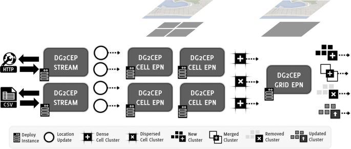

  

  Overview of DG2CEP distributed event processing architecture

• 2 Detection of grid cells which have become dense or sparse over time (Cell EPN);

• 3 Correlate dense and sparse cells with existing grid clusters to create or modify them (Grid EPN).

Each stage of the algorithm can be deployed concurrently to distribute the workload. Distributed instances are interconnected through a publish/subscribe middleware that provides uncoupled communication between each stage. For instance, a deployed instance can subscribe to position data of a specific spatial range to only handle events from that region, as shown in Fig. 2, where each Cell EPN only consume events from specific Location Update range.

4.1 Stream receiver EPN

DG2CEP’s first stage, Stream Receiver, is responsible for continuously receiving and mapping incoming moving objects location as LocationUpdate events. Moving objects periodically inform their location by sending the following data: 〈id, lat, lng, t〉, where id is the moving object’s identifier, lat and lng are their current position (latitude and longitude values, respectively), and t is the timestamp the data was sampled.

Incoming data stream tuples are mapped to a grid cell 〈i, j〉 to avoid the pairwise distance comparison between them. By doing so, the algorithm can rely only on counting the number of location updates in each grid cell to discover dense and sparse cells, that will constitute the spatial clusters.

Thus, following this idea, the monitored spatial domain (a rectangular region defined by [lat_min,lat_max] and [lng_min,lng_max]) is divided into a grid G of grid cell size $\frac {\varepsilon }{\sqrt {2}} \times \frac {\varepsilon }{\sqrt {2}}$. The choice for this respective grid cell size is to guarantee that the maximum distance between any two location updates within the grid cell is ε, similar to DBSCAN ε–Neighborhood, as shown in Fig. 3. Thus, G is segmented in the following intervals:

• $i \rightarrow \left [{lng}_{min}, {lng}_{min} + i \times \frac {\varepsilon }{\sqrt {2}}, \ldots, {lng}_{max}\right ]$ and

  Fig. 3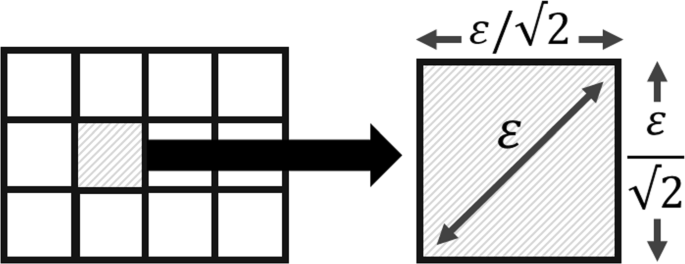

  

  Example of DG2CEP $\frac {\varepsilon }{\sqrt {2}} \times \frac {\varepsilon }{\sqrt {2}}$ grid cell division

• $j \rightarrow \left [{lat}_{min}, {lat}_{min} + j \times \frac {\varepsilon }{\sqrt {2}}, \ldots, {lat}_{max}\right ]$

for longitude and latitude respectively.

Algorithm 1 describes the required steps to translate incoming data into LocationUpdate events. DG2CEP stores the grid intervals in a static data structure, which allows efficient retrieval of the corresponding cell index. It is possible to directly compute the cell index using the formula: $\left \lfloor \frac {lat - {lat}_{min}}{\varepsilon \sqrt {2}} \right \rfloor$ and $\left \lfloor \frac {lng - {lng}_{min}}{\varepsilon \sqrt {2}} \right \rfloor$, where lat and lng are the position data location, and lat_min and lng_min are the domain region’s lower boundaries. This formula represents the roughly, rounded, number of $\frac {\varepsilon }{\sqrt {2}}$ units required to index the incoming position data. Finally, DG2CEP emit a LocationUpdate event that enriches the incoming position data 〈id, lat, lng, t〉 with its corresponding grid cell i and j index.

This algorithm can be expressed in CEP by using the project and enrich primitives. Project retrieves the existing data, while enrich adds the cell index, creating a LocationUpdate event. An EPA with this continuous query can be deployed in parallel without any collateral effects due to the stateless nature of such primitives.

4.2 Cell EPN

DG2CEP second stage, Cell, is responsible for discovering dense and sparse grid cells from incoming LocationUpdate events. Thus, first, it uses a communication middleware to subscribe to LocationUpdate events that are within a spatial range. By subscribing to events that only occur in such region, it is possible to distribute the workload among instances, as shown in Fig. 2.

4.2.1 Dense cell discovery

Algorithm 2 describes how DG2CEP detects the formation and dispersion of dense and sparse cells. Each grid cell gets assigned a density value, which is the number of unique LocationUpdate events mapped to the cell within the past Δ time units.

LocationUpdate events assigned to a cell are all within ε distance (ε-Neighborhood) apart from each other since the cell length is $\frac {\varepsilon }{\sqrt {2}}$, which means that the maximum distance between two moving objects in the same grid cell is $\frac {\varepsilon }{\sqrt {2}} \times \sqrt {2} = \varepsilon$. Hence, to calculate the grid cell density the algorithm retrieves all unique LocationUpdate events in the data stream, within a Δ period, that are in the incoming event grid cell index (e.g., G_ij).

The grid cell structure can be translated to CEP as context partitions that segments the incoming LocationUpdate event stream based on its (i, j) index. For example, Code ?? creates such context partition (CellContext) following this definition. Each stream partition will only consider events that are in the same grid cell, i.e., those that have the same i and j index.

Following this idea, the cell density value can be easily computed in CEP by taking advantage of the CellContext partition. Precisely, whenever it receives a LocationUpdate event it can use its (i, j) index to select the appropriate context partition sub-stream, followed by the event timestamp t and to slide and retrieve only events that are within a given period. The resulting sub-stream slides the context sub-stream and mitigating the issues related to batching, where spatially close data were placed in different batches, since the window will slide accordingly to the analyzed event.

Likewise, core moving objects in DBSCAN, grid cells whose density value is greater than or equal to minPts are considered dense and classified as a core. Therefore, to discover core cells, DG2CEP filter the CellContent event stream to identify events whose density value is equal or higher than minPts. This simple task can be continuously and timely done in CEP through the usage of the filter and project primitives. If the analyzed CellContent event density surpass minPts, the EPA produces a derived complex CellCore event.

Analogously to DBSCAN, in DG2CEP, the most straightforward cluster is formed by the combination of a core grid cell ($\mathcal {C}$) and its neighboring border cells ($\mathcal {N}$), which are then further visited in a later part of the algorithm. Thus, DG2CEP needs to enrich the CellCore events with its adjacent border cells to create a complex event named DenseCellCluster, to be further expanded. This can be done by joining incoming CoreCell event $\mathcal {C}$ with existing CellContent events (in the Δ period). As a result, the continuous query produces a complex DenseCellCluster event, which contains the CellCore event ($\mathcal {C}$) and the resulting collection set containing its neighboring cells ($\mathcal {N}$).

The degree of parallelism of the Cell processing stage is associated to the number of grid cells, that is, this stage can process in parallel one event for each grid cell index since its computation is based on each grid cell. This upper limit is used to avoid inconsistency. For example, consider that two LocationUpdate events from different moving objects, but mapped to the same grid cell 〈i, j〉 index, are being processed in parallel.

In such scenario, due to the stateful nature of the count primitive, it may miss the other LocationUpdate that is being processed in parallel. However, it is important to note that this degree of parallelism refers to each EPA and not the entire EPN, that is, several events with the same cell index can coexist in the EPN, but at different EPAs pipeline stages.

4.2.2 Sparse cell discovery

Cells become sparse when its density drops below minPts. This can happen whenever moving objects change their grid cells or if they stop updating their location. To detect the first situation (cell change), DG2CEP stores the latest grid cell of each moving object in a map $\mathcal {L}$, as shown in Algorithm 2. For instance, if the most recent position of a moving object with id equal to 7 was in grid cell (4,9), then $\mathcal {L}(7) = (4, 9)$. DG2CEP checks if a moving object has changed it cell by comparing if its incoming LocationUpdate event cell index differs from its than its previous position, i.e., if $\mathcal {L}(id) \neq \langle i, j \rangle$, where i and j are the current location update cell indexes.

This situation can be timely verified by an EPA continuous query using the CEP sequence and filter primitives. To do that, first, the EPA employs the select primitive to extract consecutive LocationUpdate events. Then, it filters the event if their grid cell index differs. As output, the EPA produces a complex CellRecheck event containing the previous grid cell of the incoming moving object. If the density value of a cell is less than minPts the continuous query generates a complex DispersedCellCluster event to indicate that it has become sparse.

Moving objects can also stop sending LocationUpdate events, which can lead to a cell cluster becoming sparse even though moving objects did not change cells. DG2CEP can detect such situation through the usage of CEP sequence and absence primitives combined with a Δ sliding window period. This EPA verifies if a previous DenseCellCluster event in a grid cell (i, j) is not followed by another DenseCellCluster event within a Δ period. The absence of this event throughout this period indicates that the number of location updates mapped to the cell dropped to less than minPts and that it is no longer a cell cluster. By setting up a Δ time window value equal to the moving objects’ location update frequency, DG2CEP makes sure that all location updates have been considered.

Similar to the dense cell discovery, the degree of parallelism for the sparse detection phase is associated with the number of context partitions (grid cells). It can process an event for each grid cell in parallel without having collateral effects. Further, the sparse detection algorithm can be processed in parallel with the dense cell discovery one.

4.3 Grid EPN

So far DG2CEP is only detecting the formation and dispersion of individual cell clusters. To detect clusters of arbitrary shapes, DG2CEP also needs to implement the successive merge and unmerge of cells, similar to DBSCAN expansion step.

The Grid EPN is responsible for handling cell cluster and disperse events to create, destroy, and evolve grid clusters. In terms of CEP workflow this boils down to merging and expanding grid clusters when receiving DenseCellCluster events, while removing cells from, and occasionally splitting or destroying, existing grid clusters when receiving DisperseCellCluster events.

Analogous to DBSCAN, where clusters are collections of density-connected core and border moving objects, in DG2CEP, grid clusters are the resulting combination of one or more adjacent DenseCellCluster events. In turn, each DenseCellCluster event contains a core grid cell and its corresponding neighbors.

To represent a grid cluster, DG2CEP uses CEP’s streaming relation concept, a shared memory structure that can be used within different continuous queries. By storing the grid clusters in such relation, DG2CEP can add, update, and remove clusters from different EPAs. The cluster streaming window schema is defined as follow: 〈cid, x, y〉, where cid is the cluster identifier and x and y are the core cell cluster index¹.

To exemplify this schema, consider the Grid Clusters (GC) streaming window illustrated in Fig. 4. Here, a grid cluster with cid=15 contains two core cells, with indexes (5,9) and (5,10), while the cluster with cid=16 contains three core cells: (3,3), (4,2) and (4,1). The relation window only index the grid clusters core cells, since its border ones can be easily retrieved through the core cells adjacency. The remaining subsections discuss how to build and manage such clusters.

Fig. 4

An example of the Grid Clusters streaming window

4.3.1 Grid add, update, and merge

Algorithm 3 describes how DG2CEP expands DenseCellCluster events to create and evolve grid clusters. First, DG2CEP unwrap the complex event and adds its core and border cells to a grid G. Before further processing the event, it has to verify if it is creating, augmenting, merging, or just updating an existing grid cluster. We decide to untangle these different cases by checking for a cluster update since it is the most frequent situation, i.e., when a cell cluster updates the position or number of moving objects.

DG2CEP updates an existing cluster if it contains a core cell which index is equal to the incoming cell G_ij. If positive, it output a GridCluster event with the cluster ID and a UPDATE tag. However, when no existing clusters contain G_ij, it means that either the core cell can form a cluster or can be merged into an existing one. Nevertheless, in both cases, the conclusion of such operation is a new cluster, either one with this single cell or the result of the merged one. Thus, DG2CEP insert a new grid cluster in the streaming window containing such cell. Subsequent EPAs will process this information to filter out each case.

To avoid inconsistency issues when processing events in parallel, a lock is applied for this rule for each cell index. Thus, the degree of parallelism associated with this EPA is also the number of cells. While an event with cell index G_ij is being processed, subsequent events with index i and j are queued, while events with different cell indexes can be processed in parallel.

Part of this algorithm is described in CEP in Code ??. This EPA uses the merge primitive to atomically update or insert a core cell in the GC relation if there is a cluster that contains the incoming core cell i and j index. If there is a match the EPA outputs a complex GridClusterUPDATE event by using the corresponding cluster id. Otherwise, the EPA insert a new entry to the GC streaming window containing the incoming core cell indexes and a newly generated cluster id.

Now, DG2CEP needs to process the newly created grid cluster. Thus, first, DG2CEP identify if there are adjacent grid clusters to the newly created one. This task can be done by querying the GC streaming window using each adjacent (border) cell index. If the EPA returns an empty set $\mathcal {N}'$ of neighbors, i.e., if there are no grid clusters that are neighbors of the newly dense cell, then there is no merge process. However, if the $\mathcal {N}'$ set is non-empty, DG2CEP will merge the grid cluster by uniting the neighboring grid clusters. This is due to the newly created grid cluster serving as a link to connect all its neighboring grid clusters. To efficiently merge the cluster, DG2CEP needs to update all core cells of adjacent grid clusters to the new id.

To exemplify this process, consider the scenario shown in Fig. 5. The GC streaming window contains tree grid clusters. Now, consider that the incoming DenseCellCluster event is the hashed cell with index equal to (4,4). DG2CEP first verifies if the incoming cell event is already contained within a given grid cluster. In this case, it is not located in any grid cluster. Thus, it creates a new grid cluster using the incoming event cell and a unique ID, e.g. 17. Then, it looks for adjacent grid clusters in its neighboring cells. In this case, there are three adjacent grid clusters. The resulting of this merge is a single grid cluster with ID 17 and composed by the union of all adjacent grid clusters (12, 14, and 16) since the incoming core cell interconnects them.

Fig. 5

Sample scenario of merging grid clusters

Finally, in addition to the event semantics (e.g., add, merge), the grid cluster output should also include the core and border cell contents. DG2CEP build such output by consuming the GridCluster event. The resulting set is wrapped alongside the event semantic in a complex GridClusterOutput event. This event is intended to be consumed by endpoint applications or to be further processed by other EPAs continuous queries.

4.3.2 Grid disperse

When a cell cluster disperses, i.e., when receiving a DisperseCellCluster event, it is necessary to timely reflect this change in the GC streaming window, as described in Algorithm 4. First, DG2CEP identify the cluster that contains the dispersed cell. This is done by comparing the incoming disperse cell index to the grid clusters’ core cells indexes in GC.

Incoming DisperseCellCluster events are joined with the GC relation by correlating the disperse cell indexes. Using the dispersed cluster id, DG2CEP extract its core cells. By doing so, it can verify if the cluster in question should be destroyed or split after removing the dispersed cell.

After extracting the cluster core cell, DG2CEP only needs to identify and handle possible residual (e.g., split) clusters. A list of clusters $\mathcal {R}$ is created to hold the residual clusters. Each member of this list is a set r (residual cluster) whose elements are the core cell.

To verify if a core cell belongs to a residual cluster, DG2CEP check if a residual cluster contains an adjacent cell to the one being analyzed. If it does the remainder core cell is added to the residual cluster, otherwise, a new residual cluster is created with this cluster. After this step, the cluster containing the dispersed cluster is deleted. Then, each of the residual clusters is reinserted in the streaming window. This is done by generating a new cluster id with the combination of the core cells belonging to this residual cluster. If there is no residual grid cluster, i.e., $\mathcal {R} = \varnothing$, a destroyed semantic is emitted to indicate that the grid cluster has faded.

4.4 Discussion

By using an $\frac {\varepsilon }{\sqrt {2}} \times \frac {\varepsilon }{\sqrt {2}}$ square shaped grid cells, DG2CEP reduces the problem to counting the number of moving objects that fall into each cell. Similar to DBSCAN, in DG2CEP still needs to expand the core grid cells, i.e., those that are dense w.r.t. the minPts parameter, but this process is more straightforward and efficient as they are disposed in a grid. Hence, the main performance factor is not anymore the number of moving objects location updates but instead the number of grid cells g, or context partitions, which solely depends on ε.

The tuning of the ε parameter and the frequency of location updates sent by moving objects for a concrete application is very complex, and requires expertise in the application domain [2, 6]. We assume that such information is known in advance. Regarding the sliding window size (Δ), it has a direct relationship with the expected frequency of the moving objects’ location update. Ideally, Δ should be large enough to slide and retrieve the latest location updates of every moving object being considered.

Regarding algorithmic complexity, it is hard to calculate DG2CEP computational cost given its event-based nature. Considering the worst case scenario, the computational cost is determined by its longest event path, i.e., a location update that passes through all EPAs stages. Thus, in this case, the computational cost of DG2CEP per location update is:

$$\begin{array}{*{20}l} DG2CEP &=\, \mathcal{O}(SR) + \mathcal{O}(Cell) + \mathcal{O}(Grid) \\ &=\, \mathcal{O}(\lg g) + \mathcal{O}(1) + \mathcal{O}(g) \\ &=\, \mathcal{O}(g) \\ {where}~ g & \text{ is the number of grid cells}. \end{array} $$

The Stream Receiver (SR) EPN cost is associated with g, the number of grid cells (context partitions). Using a static grid structure that holds intervals, such as Segment Tree, DG2CEP can identify the grid cell indexes in $\mathcal {O}(\lg g)$. The computation of an approximation cell index can also be done in constant time, $\mathcal {O}(1)$, since it can be directly computed through the location update latitude and longitude values, roughly the number of $\frac {\varepsilon }{\sqrt {2}}$ units required to index this position.

After mapping the location updates to a cell, DG2CEP checks if the given cell density is greater or equal to minPts. When this happens, the algorithm retrieves its adjacent neighbors and builds a complex DenseCellCluster event to be further expanded. Further, it also checks if the previous cell of the moving object has dispersed. In both cases, for detecting dense and sparse cells, the computation can be done in constant time since it involves basic operators.

Finally, the last algorithm stage, Grid EPN, consumes the dense and disperse cell events. The DenseCellCluster event triggers the EPA to check if the incoming dense cell will form a new grid cluster or is part of an existing one. This process requires an iteration over the existing grid clusters cells. In the worst case, each cluster could be a single cell in the grid, which would require an iteration over all g grid cells. Hence, its computational cost is $\mathcal {O}(g)$. For DisperseCellCluster events the process is similar. Here, the worst case scenario is that a cell becomes sparse in a grid cluster composed of every cell. In this case, the algorithm would need to iterate over all the g grid cluster cells to discover residual clusters. Thus, its computational cost is also $\mathcal {O}(g)$. Therefore, considering all the aforementioned steps, the cost for the entire DG2CEP algorithm pipeline is $\mathcal {O}(g)$.

However, it is important to note that DG2CEP worst-case scenario is unlikely to occur for all events in the stream. It would require all location updates in the Δ time window to have their corresponding moving objects located in dense cells. In most cases, most location update events will pass only through the SR and stop at the Cell stage, which has a low cost.

4.5 Limitations

While DG2CEP’s counting approach of grid cells gives a performance advantage over distance comparison, it also entails what we call the answer loss or blind spot problem: the difficulty to detect a dense grid cluster when spatially close location updates are mapped to adjacent grid cells [22, 23, 36]. The answer loss problem happens in any grid-based approach because the spatial domain is segmented in ε square shaped cells, and moving objects that are ε distance apart from each other may be mapped to different cells, not contributing to the required minPts density. For example, suppose that minPts=4 and the cells have the following location updates illustrated in Fig. 6. In this case, no cell would be dense since their density is below the minPts threshold even though there is a definite high density of location updates in the picture close to the borders of all 4 cells.

Fig. 6

Blind Spot Scenario in DG2CEP for minPts=4

It is possible to compare DG2CEP’s and DBSCAN’s clustering results. Considering that there are no answer loss, DG2CEP clustering results are a superset of DBSCAN one. Suppose that a grid cluster in DG2CEP has c core and b border grid cells. Hence, all location updates in the c core grid cells would also be included in DBSCAN result since they are all within the ε distance. DG2CEP default expansion includes all the border grid cells. Therefore, in the worst-case scenario, the neighbor grid cells should not be included, since their content is beyond the ε distance. To exemplify this issue, consider the scenario illustrated in Fig. 7, with minPts=4 and a grid cluster with two core and eight border cells.

Fig. 7

DG2CEP result as a superset of DBSCAN one

The number of location updates detected by DG2CEP in this cluster would be |c|+|b|=12, where |c| and |b| are the number of location updates placed in the cluster’s core and border cells respectively. This result is a superset of DBSCAN’s outcome, which is 9 location updates. This clustering error is limited by following equation: |b|×(minPts−1). This means that, since DG2CEP includes all the content of neighbors partitions, in the worst-case scenario, all their moving objects are not within ε distance of the core partition. However, these partitions are limited by minPts, otherwise, they would have been included as core partitions.

5 Answer loss heuristic

In this section, we present a heuristic to address the answer loss subproblem [22, 23, 36]. This subproblem happens in DG2CEP, and other grid-based approaches, due to the discrete division of the spatial domain into grid cells, which can lead to spatial close locations updates being mapped to different cells. Although moving objects are close w.r.t. ε and minPts, a cluster may not be detected since they objects may be mapped to different grid cells, as seen in Fig. 6.

5.1 Transient heuristic

To address the answer loss subproblem, while retaining DG2CEP counting semantic, we propose a density heuristic that logically divides each grid cell into $\mathcal {S}$ inner slots (strips), in both directions, horizontal and vertical. The overall idea is to consider the distribution of moving objects inside these adjacent cell slots when calculating the cell density. Then, the density function counts the number of location updates in those inner slots in a way that slots closer to G_ij have a higher weight than those that are more distant.

Each location update mapped to a grid cell G_ij is also mapped to a horizontal and vertical slot index s, such that s varies from 0 to $\mathcal {S} - 1$, the first and last slot respectively. This operation can be effectively done in constant time during DG2CEP Stream Receiver EPN phase by comparing the location update position with the width and length size of each slot.

Since the heuristic considers moving object in adjacent cells when computing a given cell density, as a collateral effect, it can lead to a cluster that does not exist. To mitigate this issue, the idea is to apply the heuristic only to cells whose density fall within minPts and an even lower boundary transientPts. Such cells are called transient grid cells.

To apply the heuristic, DG2CEP needs to analyze the neighborhood of the transient grid cell. To do so, it updates the density function to consider the inner density of neighboring cells, as shown in Fig. 8. We use a decay weight function that counts the number of location updates inside each inner slots of each neighboring cell in such a way that slots closer to G_ij receive a higher weight. The heuristic density is the sum of the location updates’ placed in each slot with their corresponding weight. Closer slots indexes vary according to the position of the neighboring cell, as shown by darker tones in Fig. 8.

Fig. 8

Density neighborhood of a cell G_ij. Note that the neighbor’s closer inner slots is relative to the position of G_ij

The heuristic density function is described as:

$$d(G_{ij}, N_{\varepsilon}(G_{ij})) = |G_{ij}| + \sum_{n \in N_{\varepsilon}(G_{ij})} \left (\sum_{s=0}^{\mathcal{S}} n_{s} \times w_{s} \right), $$

where |G_ij| is the number of location updates contained in G_ij, n∈N_ε(G_ij) is a adjacent cell neighbor, $\mathcal {S}$ is the total number of inner slots, n_s is the number of location updates in the s^th slot index of a neighboring cell n, and w_s is the s^th decay weight.

The density heuristic can use two weight functions, a linear and an exponential one, as illustrated by Fig. 9. The linear decay weights can be computed as $w_{s} = 1 - \frac {s}{\mathcal {S}}$, where s is the given grid cell inner slot index. For example, considering $\mathcal {S} = 4$, the slots weights are w₀=1, w₁=0.75, w₂=0.50, w₃=0.25 and w₄=0. Thus, when computing the cell density, the number of location updates in the first slot contribute directly, since they are multiplied by 1, while those placed in the last slot does not add to the cell density.

Fig. 9

Linear and exponential weights for $\mathcal {S} = 4$ inner slots

Likewise the linear weight, the exponential decay weights can be computed as w_s=k^s, where k is a number between 0 and 1 such that $k^{\mathcal {S}} \approx 0$. Based on this definition, k varies accordingly to the number of inner slots $\mathcal {S}$. For example, considering that cells have $\mathcal {S} = 4$ inner slots, k value is approximately 0.3162, i.e., 0.3162⁴≈0, while for grid cells that have $\mathcal {S} = 10$ inner slots, k is approximately 0.6309, since 0.6309¹⁰≈0.

5.2 Usage and limitations

By applying the discrete weight function to the neighboring cells inner slots, the proposed heuristic can detect several answer loss clustering scenarios. For example, consider the clustering scenario of Fig. 10a and parameters $\mathcal {S} =4$ and minPts=4. Since the analyzed grid cell density is 2, thus less than minPts, DG2CEP would not detect the cluster. Using the heuristic, with a linear weight decay, the computed density will be 2+(1×1)+(4×0.75)=5≥minPts, thus, the cluster would be detected. An exponential decay weight will also detect this cluster, since the density would be 2+(1×0.3162⁰)+(4×0.3162¹)=4.26≥minPts.

Fig. 10

Cell configuration scenarios. In a the scenario forms a cluster, while in b it does not

On the other hand, as a collateral effect of considering moving objects of neighboring cells when calculating the cell density, the proposed heuristic would detect a non-existing cluster (a false positive) in some situations, as illustrated in the cell configuration of Fig. 10b, for $\mathcal {S} = 4$ and minPts=4. In this scenario, DG2CEP would correctly not detect the cluster, since the cell density is 1. However, the linear weight decay would wrongly detect the cluster, since the cell density in this case would be 1+(1×1)+(1×0.75)+(2×0.5)+(1×0.25)=4≥minPts. Nevertheless, in this scenario, the exponential weight decay would correctly not detect such cluster, since the computed density would be 1+(1×0.3162⁰)+(1×0.3162¹)+(2×0.3162²)+(1×0.3162³)=2.54≤minPts.

To mitigate the heuristic collateral effect of detecting non-existing clusters, we propose only to apply the method in transient cells, i.e., those whose density is lower than minPts, but higher than a transientPts threshold, where transientPts≤minPts. By using a lower-bound threshold, we can restrict the heuristic application to almost dense grid cells. For example, consider a transientPts=2 threshold in the clustering scenario of Fig. 10b. In this configuration, the linear weight heuristic will correctly not detect the cluster, since the cell density would be 2. In addition to mitigating false positive answers, transient cells also reduce the overall heuristic computational cost, since the heuristic will only apply to grid cells whose density are within the transient interval.

6 Evaluation

DG2CEP was evaluated using a real-world data stream generated by the bus fleet of the city of Rio de Janeiro². The evaluation had the following goals. First, measure the elapsed time required by DG2CEP to detect the formation, dispersion, and evolution of spatial clusters when compared to the baseline DBSCAN off-line algorithm. Second, measure the elapsed time required by the well-known grid and batch-based D-STREAM [21] algorithm to indirectly compare it to DG2CEP. Further, measure how the elapsed time varies according to the number of moving objects and partition sizes ε.

We also evaluated the heuristic-enhanced DG2CEP under different transient thresholds. Here, the goal was to compare the heuristic version with basic DG2CEP and DBSCAN. Also, we evaluate if the number of inner slots impacts the number of clusters found.

Finally, the evaluation measured how similar DG2CEP’s clustering result is to DBSCAN throughout the entire data stream using a second-by-second analysis. By doing that, we aim to verify if DG2CEP’s clustering result can keep up” to DBSCAN by measuring their similarity throughout the data stream. For this we used the Rand Index [37], which measures the similarity between clusters, considering the number of true positive, true negative, false positive, and false negative moving objects placed in a given cluster.

6.1 Implementation

DG2CEP was implemented using Java and several open source libraries. The reason for using Java is due to the numerous libraries, frameworks, and middleware platforms available in this language. For example, we opted to use the Esper CEP Engine [31], one of the leading open source CEP engines, which is available as a Java library. Esper provides a continuous query CQL-like declarative language that supports CEP’s primitives. We implemented DG2CEP event processing network as a network of Esper’s continuous queries.

DG2CEP also uses the SDDL communication middleware [38] to interconnect the different parts of the EPN. SDDL provides publish/subscribe communication with real-time guarantees for local, mobile, and cloud instances, based on the OMG DDS standard. It is also written in Java and uses OpenSplice, an open source implementation of the DDS standard.

Each DG2CEP distributed instance also implements a wrapper for life-cycle management and interaction with the Esper CEP Engine, that can dynamically create and destroy EPAs. These functions are implemented as commands, enabling EPAs to be deployed and interconnected locally or remotely by dynamically generating the necessary listener and subscriber routines to receive or route input/output events. This strategy enables DG2CEP instances to be as flexible as needed. For example, one can deploy the entire EPN in a single machine, or subdivide into different machines.

6.2 Data stream

We crawled the data stream from the data.rio open platform and obtained a dataset containing the trajectory data for the city’s 11,324 buses for one hour (from 17:30 to 18:30) for the week of July 12^th to 19^th of 2016. We choose the rush hour period because it contained the most substantial throughput, and probably the largest number of spatial clusters.

While crawling the data stream, we learned that, on average, each bus update its location every 60 s. Hence, considering 11,234 buses, each second contains in average 187 location updates. With the intent to increase the data stream volume, we augmented the data stream using linear interpolation between buses location updates in such a way that a location update is emitted every second for every bus. More precisely, between two consecutive buses location update points we generated additional location updates on the direct line between these two points. Using this method, we produced four resulting data streams with 2500, 5000, 7500, and 10000 location updates events per second.

The reason for choosing such numbers is to reflect the size of real-world bus fleets in metropolis [39]. For instance, New York City has 5700 buses, while Los Angeles has 2328 [40]. Further, as said, moving objects does not necessarily send an update every second. By augmenting the data stream, we aim to evaluate if DG2CEP can scale and handle higher throughputs. For example, a data stream with 7500 location updates per second can represent a moving object fleet of 60×7500=450,000 vehicles, where each individual moving object update its position every 60 s.

We established the data stream ground truth clustering results by computing DBSCAN³ at every second of the one hour. As a result, we have a snapshot of the spatial clusters and their content (moving object’s location updates) that appears at every second of the data stream. This is an expensive computing task. It took more than 24 hours to compute the second-by-second ground truth results. Using this information, we are able to evaluate how close DG2CEP is to the optimal off-line clustering result.

6.3 Answer loss

The first experiment evaluates the proposed heuristic impact in the DG2CEP performance concerning similarity and number of wrongly detected and undetected clusters. We start by evaluating the proposed heuristic since the later experiments will utilize the heuristic. Using the heuristic-enhanced DG2CEP, the evaluation had two goals:

• Measure the similarity of clusters found, when compared with the original DG2CEP and the baseline DBSCAN off-line algorithm. Furthermore, investigate how these results vary with different transientPts values that define transient cells.

• Investigate if the number of correct and incorrect clusters found and their similarity with DBSCAN vary when using a different number of inner slots s.

The second-by-second DBSCAN ground-truth result enabled us to compare and measure the effect of the proposed heuristic clustering with the original grid-based DG2CEP and DBSCAN output. Whenever the enhanced-heuristic DG2CEP discovers a cluster, we take a snapshot of its content (moving objects’ location updates) to analyze at a later time. Using this information, we compare the clusters found with their counterparts in the ground-truth log.

A cluster C is discovered in DG2CEP at timestamp t if DBSCAN ground-truth log contains a cluster D, in the same timestamp, such that the overlap between them is higher or equal to 50% (C∩D≥0.5), i.e., the cluster found in DG2CEP contain at least 50% of the content of the ground-truth cluster. Such threshold 50% comes from the MONIC clustering transition model [41], which states that a cluster is a match only if it contains at least half of its members.

If the heuristic wrongly detects a cluster, i.e., no similar cluster exists in DBSCAN log, hence it is marked as false positive (FP). All clusters not detected by the heuristic but present in the ground-truth log are marked as false negatives (FN). By comparing these metrics, the percentage of incorrectly clusters found (FP) and missed clusters (FN), to the total number of clusters in the ground-truth log, we can measure DG2CEP effectiveness of handling the answer loss problem.

6.3.1 Experiment parameters

Since the primary interest of this experiment is to measure the heuristic impact in DG2CEP we fixed a set of values. First, we used a data stream throughput of 5000 location updates per second, a grid size of ε=100 meters, and minPts=20. We also set DG2CEP’s sliding window to be Δ=60 s, i.e., we consider the location updates received within the last 60 s.

We considered transientPts thresholds ranging from 90% to 30% of minPts. Since minPts=20, we evaluate the following transientPts thresholds: 18, 16, 14, 12, 10, 8, and 6. We chose to vary the threshold until it is 30%, because lower values tend to produce more false positive clusters due to the heuristic collateral effects.

Finally, we evaluate the impact of inner slots ($\mathcal {S}\!=10$). Hence, since ε=100 m, each inner slot $s = \frac {100}{\mathcal {S}}$ width is 10 meters. We choose these values considering that the GPS accuracy is approximately between 10 to 20 meters. However, in this experiment, we also evaluate if the total number of slots $\mathcal {S}$ impact the similarity of clusters found. For this test, we have considered the following number of slots: 10, 50, and 100. As a result, we have the configuration shown in Table 1.

Table 1 Parameters for DG2CEP’s Heuristic Experiment

6.3.2 Experiment setup

We executed these experiments in the Microsoft Azure Cloud platform using two virtual machines running Ubuntu GNU/Linux 14.04.3 64-bit and the OpenJDK 1.7.91 64-bit Java runtime. One of the virtual machines replayed the data stream, while the second one contained an instance of DG2CEP with its entire EPN. The virtual machines were interconnected through a Gigabit link/bus and had the following hardware configuration:

• Intel Ⓡ Xeon CPU E5-2673 v3 @ 2.40 GHz

• 28 GiB Memory RAM

6.3.3 Result and analysis

In this subsection, we present and discuss the evaluation results. Each experiment was run 10 times, and the error bars in the graphs represent a 95% confidence interval.

Figure 12 illustrates the average percentage of missed clusters (False Negative – FN) and incorrectly clusters found (False Positive – FP) of the proposed heuristic in DG2CEP at a given second, when compared with the ground-truth clustering results in the specified second for a one-hour test period and parameters ε=100, minPts=20, and $\mathcal {S}= 10$. The two line graphs illustrated by Fig. 12a and b represent the values obtained when evaluating the heuristic with linear and exponential weights respectively.

According to the linear weight graph, Fig. 12a, the transientPts thresholds that yielded the best tradeoff results were 60% and 50% of minPts. These thresholds reduced the number of missed clusters from 80% to 23.57% and 15.32%, respectively, with a collateral effect of incorrect clusters of 13.51% and 19.05%, respectively. More specifically, using such parameters, a single heuristic-enhanced DG2CEP instance was able to provide in real-time at a given second a clustering result that is 84.68% similar to the off-line DBSCAN result at that second.

To exemplify such results consider the graphs illustrated by Fig. 11, which shows the similarity between the clusters found of DBSCAN and DG2CEP, using a linear heuristic and transientPts=50%. Each marker (in red) represent a cluster centroid. As can be seen, clusters detected in real-time by the on-line DG2CEP algorithm are located in a similar position to their counterpart in off-line DBSCAN.

Fig. 11

Graphical comparison between the off-line DBSCAN clustering result and DG2CEP on-line clustering result

The heuristic exponential weight graph, Fig. 12b, presented better results as transientPts decreases. This illustrates that exponential weights is more tolerant of collateral effects. For example, the number of incorrect clusters results is 4.47% for a transientPts equal to 30% of minPts. However, for this parameter, the heuristic reduced the number of cluster not detected due to the answer loss problem, from 80% to 31.51%, instead to 13.51% when using linear weights.

Fig. 12

Percentage of Incorrectly Detected (FP) and Undetected Clusters (FN) in heuristic-enhanced DG2CEP (for ε=100, minPts=20, and $\mathcal {S}=10$). a Linear Weight b Exponential Weight

With respect to the relationship between the total number of cell subdivisions $\mathcal {S}$ and the heuristic results, Figs. 13 and 14 shows how the number of undetected clusters (false negative) and incorrectly clusters found (false positive) vary for different number of cell slots when using the heuristic linear and exponential weight respectively for parameters ε=100 and minPts=20.

Fig. 13

Relationship between heuristic results and the total number of cell slots subdivisions $\mathcal {S}$ for linear weights. a False Positive b False Negative

Fig. 14

Relationship between heuristic results and the total number of cell slots subdivisions $\mathcal {S}$ for exponential weights. a False Positive b False Negative

The experiments indicate that the heuristic-enhanced DG2CEP yields better results without it. Further, it shows that linear weights, combined with a smaller number of subdivision slots $\mathcal {S}$ and a transient threshold of 50%, produced the most similar clustering result to DBSCAN. Hence, for the next experiments we use a heuristic-enhanced DG2CEP with such parameters (transientPts=50 %, $\mathcal {S} = 10$, and linear weights).

6.4 Elapsed time

For this experiment, we first distinguish where new clusters appear in DBSCAN’s ground truth result. A cluster C is said to appear at second t if there is no cluster B in the previous timestamp t−1 whose intersection B∩C is higher than 0, w.r.t. the moving objects in each set. By using such information it is possible to compare DBSCAN to DG2CEP’s second-by-second clustering results Precisely, the elapsed time required by DG2CEP to detect a cluster C that appeared in timestamp t in DBSCAN is the minimum timestamp q≥t that contains a cluster D who contains at least 50 % of C elements (C∩D≥0.5).

We apply similar logic to discover where DBSCAN’s clusters dispersed. For instance, a cluster C from timestamp t−1 is said to have dispersed at timestamp t if there is no cluster B in t such that the intersection between C∩B is higher than 0, w.r.t their content (moving objects). This means that DBSCAN results show that timestamp t no longer contains a cluster that was in the previous second. Similar to the formation approach, the elapsed time required by DG2CEP to detect the dispersion of C at timestamp t is the minimum timestamp q≥t that no longer contains a cluster D whose intersection with C is higher than 0 (C∩D>0).

Finally, we do the same for cluster evolution. A cluster C evolves in DBSCAN at timestamp t when its content changes over 50 % within the previous second, that is, if exists a cluster B in timestamp t−1 where they contain elements in common, B∩C>0, but their intersection B∩C≤0.5 is less than or equal to 50 %. Hence, the elapsed time required by DG2CEP to detect this evolution is a timestamp q≥t whose contain a cluster D whose intersection with C is higher or equal to 50 % (C ∩ D≥0.5).

6.4.1 Experiment parameters

The goal of this experiment is to discover the elapsed time required by DG2CEP and D-STREAM to detect clusters under different data stream volumes. To do so, the test used three data stream throughputs: of 2500, 5000, and 7500 location updates per second.

A primary parameter of DG2CEP is the size of ε-squared grid cells (context partitions). To verify the impact of ε in the elapsed time, we further tested the experiments using three grid cell sizes: 50, 100, and 150 meters. Also, in all test runs, we set the sliding window Δ to be 60 s, to reflect the maximum interval used by the bus fleet to send their location update. Further, we fixed the value of minPts to be 20. Also, we use the proposed heuristic with linear weights, transientPts=50%×20=10, and $\mathcal {S} = 10$ subdivision slots. As a result, we have the experiment configuration shown in Table 2. We executed each experiment scenario 10 times, totalizing 90 executions.

Table 2 Parameters for DG2CEP’s Elapsed Detection Experiment

To compare D-STREAM results to DG2CEP, through DBSCAN ground-truth, we also executed the experiment configurations using D-STREAM with the following batch periods: 30, 45, and 60 s. We choose these values to understand the relationship between a lower, medium, and higher batch period.

6.4.2 Experiment setup

We executed all experiments in the DigitalOcean Cloud, where we used virtual machines running the Ubuntu GNU/Linux 14.04.5 64-bit operating system. Each experiment run was tested ten times, and error bars represent a confidence interval of 95%. All virtual machines were interconnected through a Gigabit link/bus and had the following hardware configuration:

• 4 × Intel Xeon CPU E5-2660 @ 2.20GHz

• 8 GiB Memory RAM

For this experiment, we used four different setup configurations. The first experiment setup configuration, which we called DG2CEP Single Instance, contains two virtual machines. One of the virtual machines replayed the data stream, while the second one held an instance of DG2CEP with its entire EPN. Similarly, we created a D-STREAM Single Instance setup. On this case, instead of DG2CEP, the second virtual machine contains an instance of D-STREAM.

We were also interested in measuring how the number of deploy instances impacts the experiment. For this, aside for a virtual machine to replays the data stream, we also executed the test with four and eight distributed DG2CEP instances. In the first case, here called DG2CEP 2–2, we subdivided the spatial domain into two parts and used a total of four virtual machines (two for the CELL EPN and the remaining two for the GRID EPN). In the second case, called DG2CEP 4–4, we subdivided the spatial domain into four parts. Similarly, we use four virtual machines for the CELL EPN and the other four to the GRID EPN instances.

6.4.3 Results and analysis

Figure 15 shows the elapsed time, in seconds, that DG2CEP and D-STREAM required to detect a cluster formation when compared to DBSCAN second-by-second ground-truth information. The graph indicates that the size of ε impacts the detection time. As expected, a smaller ε yields a shorter detection time when compared to the one with a large ε. A smaller ε divides the spatial domain into a larger number of context partitions, which in turn increases the cost of identifying the context partition index for each location update. However, a larger ε can also increase the detection time for cluster formation when compared to a lower ε value. The primary reason is the increase in workload in the processing network. Since more moving objects are mapped to the same grid cell, which in turn generate more events that pass through the processing network, this additional load is reflected in the detection time.

Fig. 15

Elapsed time to detect a cluster formation w.r.t. DBSCAN. a DG2CEP Single Instance b D-STREAM Single Instance (ε=100m) c DG2CEP 2-2 d DG2CEP 4-4

The experimental results show that a single instance of DG2CEP can detect cluster’s formation in a few seconds, as illustrated in Fig. 15a. The experiments also indicate that the algorithm scales with the number of moving objects, showing a linear increase in the cluster formation and dispersion detection times when increasing the data stream throughput.

For scalability, the experiment results, illustrated in Fig. 15c and d, indicates that the elapsed time required by DG2CEP to detect the cluster’s formation reduced when increasing the number of distributed instances. For instance, considering ε=100 m in a data stream scenario of 7500 location updates per second, the detected time reduced from 6.46 s (single machine) to 4.40 s for DG2CEP 2–2 configuration and to 1.83 s for its 4–4 configuration. Although more instances speed up DG2CEP process, in some cases it can lead to an increase in the elapsed time due to the overhead involved in transferring data between instances.

Concerning batch-based approaches, D-STREAM required more time to detect the cluster formation than any DG2CEP configuration under all batch periods. For example, for ε=100 m and a data stream throughput of 5000 location updates per second, it required approximately 60.38 s, 51.48 s, and 61.79 s to detect the cluster formation for batch periods of 30, 60, and 90 s respectively.

As expected, a smaller and higher batch period required more time to detect the cluster formation that a median one. With a smaller batch period the costly off-line processing is done more frequently than for the other periods, and thus more regularly D-STREAM will have to stop and compute the clusters while halting the on-line phase. Although a larger batch period also considers a higher number of moving objects in its buffer, the substantial waiting period between batches means that the cluster result is usually outdated.

The elapsed time to detect a cluster dispersion by DG2CEP and by D-STREAM for all tested scenarios is illustrated in Fig. 16. All values are higher than the ones required to detect a cluster formation. The reason is the way that dispersion of a cluster is detected in DG2CEP: a dispersion event is triggered when a moving object changes its cell or if DG2CEP does not receive a DenseCellCluster event within a Δ period.

Fig. 16

Elapsed time to detect a cluster dispersion w.r.t. DBSCAN. a DG2CEP Single Instance b D-STREAM Single Instance (ε=100m) c DG2CEP 2-2 d DG2CEP 4-4

The results also indicate a correlation between the grid cell ε size and the elapsed time required to detect a dispersed cluster. A larger ε takes more time to detect a cluster dispersion since moving objects are mapped to fewer grid cells. In particular, those moving objects help to maintain the grid cell denser for extended periods. For example, the larger a grid cell is the more it takes a moving object location update to change its cell which in turn delay the event that triggers the dispersion. Although the elapsed times to detect a cluster dispersion is higher than to detect its formation, a single DG2CEP instance is still able to detect it in few seconds as illustrated in Fig. 16a.

Similar to the experiment with cluster formation, the results indicate that the elapsed time to detect cluster dispersion also reduced when increasing the number of DG2CEP instances, as shown in Fig. 16c and d. For example, consider DG2CEP’s 4–4 distributed configuration. Considering ε=50 m in a scenario with 5000 location updates per second, the detected time reduced from 5.98 s (single machine) to 2.55 s.

D-STREAM’s batch-based approach presented significantly worst results for detecting cluster dispersion when compared to detecting its formation. The primary reason for this is that D-STREAM does not handle moving object that changes grid cells. which in turn may retain the same moving object in multiple cells. Hence, the dispersion process will take more time since more moving objects are contributing to a cell density.

As expected, D-STREAM required more time to detect the cluster dispersion than any DG2CEP configuration for all batch periods. For example, for ε=100 m and a data stream throughput of 7500 location updates per second, it required approximately 133.41 s, 117.17 s, and 141.55 s to detect the cluster formation for periods of 30, 60, and 90 s respectively. Likewise, the experiment with cluster formation, the smaller and higher batch period required more time to detect the cluster dispersion that a median one.

6.4.4 Evolution

Figure 17 shows the elapsed time, in seconds, that DG2CEP and D-STREAM required to detect a cluster evolution when compared to DBSCAN second-by-second log. The results indicate that DG2CEP was able to detect the cluster evolution under a few seconds. Furthermore, under all scenarios, the elapsed time required to detect a cluster evolution was lower than the time necessary to detect its formation and dispersion.

Fig. 17

Elapsed time to detect a cluster evolution w.r.t. DBSCAN. a DG2CEP Single Instance b D-STREAM Single Instance (ε=100m) c DG2CEP 2–2 d DG2CEP 4-4

One of the reasons for a faster detection time for evolution is that DG2CEP only needs to update the cluster content instead of either adding or merging to an existing one, which adds as overhead to the elapsed time. For instance, considering ε=100 m and throughput of 5000 location updates per second, a 2–2 DG2CEP configuration required approximately 2.1 s to detect a cluster evolution instead of 3 s for its formation.

Likewise, with cluster formation and dispersion, a single instance of DG2CEP was able to detect cluster evolutions within a few seconds, as shown in Fig. 17a. For example, considering ε=100 m, a single DG2CEP instance detected in average that a cluster has changed 50% of its element within 1.9 s, 2.3 s, and 5.28 s seconds for respectively the data stream throughput of 2500, 5000, and 7500 location updates per second.

When adding new DG2CEP instances these numbers dropped w.r.t. a single instance, as illustrated in Fig. 17c and d. For instance, in all data stream throughputs, the 4–4 DG2CEP configuration was able to reflect the off-line DBSCAN second-by-second cluster evolution result within 1.5 s. Similar to the previous experiments, D-STREAM required more time to detect the cluster evolution than any DG2CEP configuration under all batch periods.

6.5 Similarity

Beside the elapsed time, we measured the similarity between clustering results, i.e., how similar DG2CEP results are to DBSCAN’s second-by-second log. Also, we indirectly compare DG2CEP with D-STREAM, through their continuous similarity to DBSCAN.

We measured the similarity for individual clusters and the entire cluster results. For individual clusters, we estimated how similar a cluster found in DG2CEP is to its counterpart in DBSCAN. To do so, whenever DG2CEP detects a cluster we take a snapshot of its content and compare it to DBSCAN second-by-second log. Then we use the Rand Index [37] metric, which expresses the percentage of similarity between two clusters. Rand Index is a number between 0 and 1, where 1 means that the clusters are identical and 0 means that they are totally different, i.e., that they have no common moving object. Rand Index is expressed as $\frac {TP + TN}{TP + FP + FN + TN}$, where TP, TN, FP, FN, are the number of true positive, true negative, false positive, and false negative cases respectively, w.r.t. the moving objects outputted by DG2CEP and DBSCAN.

DG2CEP and DBSCAN may identify several clusters in the same snapshot. Thus, to identify the cluster D in DBSCAN that is the counterpart to C, the one discovered by DG2CEP, we need to compare C with all clusters found by DBSCAN in the snapshot. Precisely, we use C timestamp to retrieve all clusters found S in that given second. Then, we choose the cluster D with the highest Rand Index since it is the one in DBSCAN’s output closer to the cluster found with DG2CEP, that is, the counterpart cluster D is computed as a cluster that has the higher Rand Index value D= max((RandIndex(d, C)∣∀d∈S)). We call this metric Detected Rand Index (DRI), as it represents the Rand Index of a individual (detected) cluster.

We also measured how similar are the complete set of clusters detected in DG2CEP to DBSCAN. This measurement metric, which we called Complete Rand Index (CRI), compares the entire set of clusters found in DG2CEP or D-STREAM with those found by DBSCAN in a given second, not just the similarity of the detected ones. Thus, at every second, in addition to the Detected Rand Index (DRI) we consider the number of undetected clusters in the total number of clusters.

For example, suppose in a given timestamp that DG2CEP detected 3 clusters (c₁, c₂, and c₃), while DBSCAN yields 4 clusters. Then the Complete Rand Index is calculated as $\frac {dri(c_{1}) + dri(c_{2}) + dri(c_{3}) + 0}{4}$, where dri is the Detected Rand Index of the clusters detected by DG2CEP. Undetected clusters have dri=0, since the algorithm did not detect them, thus, contributing to the decrease of this similarity index.

6.5.1 Experiment parameters

To measure the data stream volume influence, the experiment was executed using two different throughputs: 2500 and 5000 moving object’s location updates per second, as described in Section 6.2. The experiment also measured the influence of different ε-squared grid cells (context partitions) sizes. Since this is a time-consuming experiment, we limited the parameter variation to 50 and 100 meters. In addition, in all test runs, we set the sliding window Δ to be 60 s, to reflect the maximum interval used by the bus fleet to send their location update. Further, we fixed the value of minPts to be 20. As a result, we have the experiment configuration shown in Table 3. We executed each experiment scenario 10 times, totalizing 40 executions.

Table 3 Parameters for DG2CEP’s Similarity Detection Experiment

6.5.2 Experiment setup

We executed all experiments in the DigitalOceal Cloud with the same four setup configurations that were described in Section 6.4.1.

6.5.3 Results and analysis

Figure 18 shows the Detected Rand Index for each experiment scenario. The graph indicates that DG2CEP’s clustering result is similar to DBSCAN. For example, in the scenario with a throughput of 5000 lu/s, the clusters found in a single DG2CEP instance (a) achieved a similarity of 93.61% and 86.54% with their counterpart in DBSCAN’s output for ε=50 and ε=100 respectively. When using a 4–4 DG2CEP instance (b), the similarity increased to 98.66% and 94.11% for ε=50 and ε=100 respectively. These results suggest that there is a relationship between the similarity and the size of the grid cell. For instance, the scenarios that used ε=50 were the ones that presented the highest similarity. The primary reason is that smaller values of ε yield smaller grid cells, which in turn have smaller areas close to the cell’s borders.

Fig. 18

Similarity of detect clusters with their counterpart in DBSCAN. a DG2CEP Single Instance b DG2CEP 4–4 c D-STREAM (ε=50m) d D-STREAM (ε=100m)

If we look at the previously elapsed time results, a smaller ε subdivides the domain into a larger number of grid cells, which in turn increases the cost of identifying the grid cell index for each moving object. Therefore, there is a trade-off when using DG2CEP: the smaller ε is, more similar will be the results of DG2CEP and DBSCAN at the cost of increasing the required computational effort and processing time.

As expected, D-STREAM results were lower than DG2CEP. This graph also indicates that the similarity of clusters found in both algorithms scales with the data stream throughput, showing a linear decrease in the similarity when increasing the data stream volume.

Figure 19 shows how the similarity of clusters found by DG2CEP and by D-STREAM evolve when compared to DBSCAN for a throughput of 5000 lu/s and ε=50 meters. Confirming our previous findings, clusters detected by DG2CEP were similar to their off-line DBSCAN counterpart. Specifically, for a throughput of 5000 lu/s and ε=50 m, the clusters detected by a single DG2CEP instance (a) presented in average a similarity of 93.61% with DBSCAN. Further, based on the line graph, we observe that DG2CEP was able to detect the clusters’ evolution throughout the entire experiment. Table 4 details the average Detected (DRI) and Complete Rand Index (CRI) for DG2CEP and D-STREAM when compared to DBSCAN.

Fig. 19

Evolution of the Detected Rand Index (“similarity”) of DG2CEP and D-STREAM with DBSCAN. a DG2CEP (ε=50m) b D-STREAM (ε=50m)

Table 4 DRI and CRI of DG2CEP and D-STREAM with DBSCAN for ε=50 m and a throughput of 5000 lu/s

Throughout the experiment, clusters found in D-STREAM presented a lower similarity to their DBSCAN counterpart than the ones detected by DG2CEP. As expected, a smaller and higher batch period presented lower similarity than one with a medium one. With a smaller batch period the costly off-line processing is done more frequently than for the other periods, and thus more regularly D-STREAM will not produce any update of clusters.

Although a higher batch period also considers a higher number of moving objects in its buffer, the large waiting period between batches means that the cluster result is usually outdated. Thus, the average batch period of 45 s presented a better balance, yielding a 66.11% similarity with DBSCAN result. It is interesting to note that the graph lines of D-STREAM contain periodic sharp edges, representing the buffering (on-line) phase of the algorithm, where the similarity constantly degrades until the next off-line phase.

The Complete Rand Index metric expresses how similar DG2CEP and D-STREAM clustering results, as a whole, are to DBSCAN at every second of the test period. As shown in Fig. 20, the results indicate that in average a single DG2CEP instance clustering result is approximately equal to 71.58% of DBSCAN’s result. When considering a distributed DG2CEP instance, these results increases to roughly 80%. In addition, the graph shows that DG2CEP was able to maintain such index throughout the test period.

Fig. 20

Evolution of the Complete Rand Index (“similarity”) of DG2CEP and D-STREAM with DBSCAN. a DG2CEP (ε=50m) b D-STREAM (ε=50m)

DG2CEP presented a higher similarity to DBSCAN results than all D-STREAM batch periods. The medium batch period (45 s) presented a higher similarity with DBSCAN when compared to the other periods. For the tested scenario, it showed a similarity of 46.06% to DBSCAN, followed closely by the smallest period (30 s), while the largest batch period (60 s) presented a similarity of only 40.39%.

An interesting result from the Complete Rand Index tests are the sudden appearance of sharply regions in the graph, such as the one from 17:10 to 17:15 in DG2CEP graph. We investigated these regions and discovered that the decrease in the similarity is due to undetected clusters by DG2CEP. Since the CRI metric compares the set of clusters found in DG2CEP with DBSCAN, an undetected cluster will decrease the similarity since its DRI is 0 and CRI is the average of detected rand index in that second.

Nevertheless, the experimental results show that DG2CEP provides better continuous clustering result than D-STREAM for all tested batch periods (30, 45, and 60 s). The results also indicate that DG2CEP was able to monitor cluster evolution and keep up with DBSCAN second-by-second result. The same cannot be said for D-STREAM due to its batch-based processing. In fact, smaller and largest batch periods (30 s and 60 s) had a worse result than the medium ones (45 s) in both indexes.

7 Conclusion

This paper presented DG2CEP, an on-line clustering algorithm that uses Complex Event Processing (CEP) [14, 15] stream-processing concepts to leverage and attain near real-time DBSCAN-like density clustering, in form of a network (EPN) of CEP declarative rules, from large position data streams. It can continuously monitor the formation, dispersion, and evolution of clusters of arbitrary size and shape. In a nutshell, DG2CEP combines density- and grid-based data stream clustering approaches and represents them as a network of CEP primitives.

The algorithm performs a DBSCAN-like [13] cluster expansion procedure but using the on-line and real-time declarative CEP primitives. The main idea behind DG2CEP is to mitigate the clustering process by first mapping the location updates to a grid, with context partitions of size $\frac {\varepsilon }{\sqrt {2}} \times \frac {\varepsilon }{\sqrt {2}}$, and then successively clustering the context partitions (grid cells) rather than the moving objects’ location updates.

Experimental results (see Section 6) indicate that DG2CEP addresses the paper main and sub research questions. The results shows that DG2CEP is able to provide an on-line and near real-time result from large position data stream w.r.t. a second-by-second off-line DBSCAN ground-truth result. For example, as illustrated in Fig. 15, in a data stream scenario of 2500 moving objects sending their position every second, a single DG2CEP instance setup detected the cluster formation in 3.33 s, 2.50 s, and 1.98 s for ε=50 m, ε=100 m, and ε=150 m respectively.

Similar results were obtained for dispersion detection. For instance, as shown in Fig. 16. Considering ε=150 m, a single DG2CEP instance was able to detected a cluster evolution within 1.78 s, 2.00 s, and 3.84 s seconds for respectively the data stream throughput of 2500, 5000, and 7500 location updates per second.

The experimental results also indicate that DG2CEP was able to maintain the results quality when increasing the data stream throughput. Considering ε=100 m, a single DG2CEP instance detected in average a cluster evolution within 1.9 s, 2.3 s, and 5.28 s seconds for respectively the throughput of 2500, 5000, and 7500 location updates per second. When adding new DG2CEP instances these numbers dropped significantly.

In conclusion, a smaller ε divides the domain into a larger number of grid cells, which in turn increases the cost of identifying the grid cell index for each moving object. Therefore, there is a trade-off when using DG2CEP: the smaller ε is, more similar will be the results to DBSCAN at the cost of increasing the required computational effort and processing time. Hence, the user has to consider his/her application’s requirements against the availability of processing resources.

However, in some situations DG2CEP may fail to identify spatial clusters, a problem known as answer loss (or blind spot) [22, 23, 36], discussed in Section 5. Although the heuristic significantly reduce the number of undetected clusters, it may still miss the detection of some clusters. For instance, considering a data stream scenario of 5000 lu/s and ε=50 m, a distributed DG2CEP setup result is approximately equal to 80% of DBSCAN off-line result at the same second, as shown in Fig. 20. Part of the remaining clusters are detected by DG2CEP in the next seconds. Hence, one of the limitations of DG2CEP on-line approach is the inability to provide an identical result to DBSCAN. By reducing the clustering problem from distance comparison, in an ε radius, to counting the number of moving objects, in a squared ε grid cell, we are losing this precision.

As future work, we plan to address the following issues. By default, each DG2CEP processing stage can be deployed in a different machine, forming a pipeline workflow. However, if a stage is overloaded, it can impact the entire system. For example, in rush hours, the stream input stage can receive a high volume of data, thus, possibly becoming a bottleneck. Motivated by this, we intend to investigate an autonomous and elastic architecture to scale DG2CEP, concerning the number of events received, by dynamically expanding and contracting the processing topology.

Also, in its current version, DG2CEP requires the setting of several parameters, such as the grid size ε, the minimum number of moving objects minPts, and the sliding window Δ. It can be complicated for the user to specify these parameters, especially because they can change over time and/or in given regions. For example, the minimum number of moving objects to form a cluster may be different based on the specified time (e.g., workhours, midnight) or in different regions (e.g., downtown, home neighborhoods. Hence, we are interested in investigating if it is possible to have a parameter free version of DG2CEP. Such version would automatically adapt and change the parameters based on its surrounding and historical data. The primary issue here is how to dynamically resize the grid cells without losing or duplicating events.

References

Dodge S, Weibel R, Lautenschütz A-K. Towards a Taxonomy of Movement Patterns. Inf Vis. 2008; 7(3):240–52. https://doi.org/10.1057/palgrave.ivs.9500182.
Amini A, Wah T, Saboohi H. On Density-Based Data Streams Clustering Algorithms: A Survey. J Comput Sci Technol. 2014; 29(1):116–41. https://doi.org/10.1007/s11390-014-1416-y.
Kargupta H, Sarkar K, Gilligan M. MineFleet: An Overview of a Widely Adopted Distributed Vehicle Performance Data Mining System. In: Proceedings of the 16th ACM SIGKDD International Conference on Knowledge Discovery and Data Mining, KDD ’10. New York: ACM: 2010. p. 37–46. https://doi.org/10.1145/1835804.1835812.
Ananthanarayanan G, Haridasan M, Mohomed I, Terry D, Thekkath CA. StarTrack: A Framework for Enabling Track-based Applications. In: Proceedings of the 7th International Conference on Mobile Systems, Applications, and Services, MobiSys ’09. New York: ACM: 2009. p. 207–20. https://doi.org/10.1145/1555816.1555838.
Zheng Y, Capra L, Wolfson O, Yang H. Urban Computing. ACM Trans Intell Syst Technol. 2014; 5(3):1–55. https://doi.org/10.1145/2629592.
Silva JA, Faria ER, Barros RC, Hruschka ER, de Carvalho ACPLF, Gama J. Data Stream Clustering: A Survey. ACM Comput Surv. 2013; 46(1):13–11331. https://doi.org/10.1145/2522968.2522981.
Khalilian M, Mustapha N. Data Stream Clustering: Challenges and Issues. In: Proceedings of the International MultiConference of Engineers and Computer Scientists 2010. Newswood Limited: 2010. p. 566–9. International Association of Engineers. ISBN: 978-988-17012-8-2. http://www.iaeng.org/publication/IMECS2010/.
Cao F, Ester M, Qian W, Zhou A. Density-Based Clustering over an Evolving Data Stream with Noise. In: Proceedings of the 2006 SIAM Conference on Data Mining. Proceedings of the 2006 SIAM International Conference on Data Mining: 2006. p. 326–37. https://doi.org/10.1137/1.9781611972764.29.
Tu L, Chen Y. Stream Data Clustering Based on Grid Density and Attraction. ACM Trans Knowl Discov Data. 2009; 3(3):12–11227. https://doi.org/10.1145/1552303.1552305.
Kranen P, Assent I, Baldauf C, Seidl T. The ClusTree: indexing micro-clusters for anytime stream mining. Knowl Inf Syst. 2011; 29(2):249–72. https://doi.org/10.1007/s10115-010-0342-8.
Yu Y, Wang Q, Wang X. Continuous clustering trajectory stream of moving objects. China Commun. 2013; 10(9):120–9. https://doi.org/10.1109/CC.2013.6623510.
Aggarwal CC, Yu PS, Han J, Wang J. - a framework for clustering evolving data streams In: Freytag J-C, Lockemann P, Abiteboul S, Carey M, Selinger P, Heuer A, editors. Proceedings 2003 VLDB Conference. San Francisco: Morgan Kaufmann: 2003. p. 81–92. https://doi.org/10.1016/B978-012722442-8/50016-1.
Ester M, Kriegel H, Sander J, Xu X. A Density-Based Algorithm for Discovering Clusters in Large Spatial Databases with Noise. In: Proceedings of the Second International Conference on Knowledge Discovery and Data Mining. KDD’96. AAAI Press: 1996. p. 226–31. http://dl.acm.org/citation.cfm?id=3001460.3001507.
Luckham DC. The Power of Events: An Introduction to Complex Event Processing in Distributed Enterprise Systems. Boston: Addison-Wesley Longman Publishing Co., Inc.; 2001.
Etzion O, Niblett P. Event Processing in Action, 1st edn. Greenwich: Manning Publications Co.; 2010.
Flouris I, Giatrakos N, Deligiannakis A, Garofalakis M, Kamp M, Mock M. Issues in complex event processing: Status and prospects in the Big Data era. J Syst Softw. 2016:1–20. https://doi.org/10.1016/j.jss.2016.06.011.
Kudyba S. Big Data, Mining, and Analytics, 1st edn. Boca Raton: Auerbach Publications; 2014. p. 325.
Roriz Junior M. DG2CEP: An On-line Algorithm for Real-time Detection of Spatial Clusters from Large Data Streams through Complex Event Processing, PhD thesis: Pontifícia Universidade Católica do Rio de Janeiro; 2017. PhD Thesis.
Roriz Junior M, Endler M, Silva e Silva F. An on-line algorithm for cluster detection of mobile nodes through complex event processing. Inf Syst. 2017; 64:303–20. https://doi.org/10.1016/j.is.2015.12.003.
Roriz Junior M, Endler M, Casanova MA, Lopes H, Silva e Silva F. In: Madria S, Hara T, (eds).A Heuristic Approach for On-line Discovery of Unidentified Spatial Clusters from Grid-Based Streaming Algorithms. Cham: Springer; 2016, pp. 128–42. https://doi.org/10.1007/978-3-319-43946-4_9.
Chen Y, Tu L. Density-based Clustering for Real-time Stream Data. In: Proceedings of the 13th ACM SIGKDD International Conference on Knowledge Discovery and Data Mining, KDD ’07. New York: ACM: 2007. p. 133–42. https://doi.org/10.1145/1281192.1281210.
Jensen CS, Lin D, Ooi BC, Zhang R. Effective Density Queries on Continuously Moving Objects. In: 22nd International Conference on Data Engineering (ICDE’06). IEEE: 2006. p. 71. https://doi.org/10.1109/ICDE.2006.179.
Ni J, Ravishankar CV. Pointwise-Dense Region Queries in Spatio-temporal Databases. In: Data Engineering, 2007. ICDE 2007. IEEE 23rd International Conference On: 2007. p. 1066–75. https://doi.org/10.1109/ICDE.2007.368965.
Han J, Kamber M, Pei J. Data Mining: Concepts and Techniques, 3rd edn. San Francisco: Morgan Kaufmann Publishers Inc.; 2011.
Rehman SU, Asghar S, Fong S, Sarasvady S. DBSCAN: Past, present and future. The Fifth International Conference on the Applications of Digital Information and Web Technologies (ICADIWT 2014) (FEBRUARY 2014). 2014:232–238. https://doi.org/10.1109/ICADIWT.2014.6814687.
Garofalakis M, Gehrke J, Rastogi R. Querying and Mining Data Streams: You Only Get One Look a Tutorial. In: Proceedings of the 2002 ACM SIGMOD International Conference on Management of Data, SIGMOD ’02. New York: ACM: 2002. p. 635. https://doi.org/10.1145/564691.564794.
He Y, Tan H, Luo W, Mao H, Ma D, Feng S, Fan J. MR-DBSCAN: An Efficient Parallel Density-Based Clustering Algorithm Using MapReduce. In: Parallel and Distributed Systems (ICPADS), 2011 IEEE 17th International Conference On: 2011. p. 473–80. https://doi.org/10.1109/ICPADS.2011.83.
Zheng K, Zheng Y, Jing Yuan N, Shang S, Zhou X. Online Discovery of Gathering Patterns over Trajectories. IEEE Trans Knowl Discov Data Eng. 2014; 26(8):1974–88.
Luckham D, Schulte R. Event Processing Glossary - Version 2.0. 2011. Accessed 08 Dec 2016. http://www.complexevents.com/2011/08/23/event-processing-glossary-version-2/. Accessed 08 Dec 2015.
Arasu A, Babu S, Widom J. The CQL continuous query language: semantic foundations and query execution. VLDB J. 2005; 15(2):121–42. https://doi.org/10.1007/s00778-004-0147-z.
EsperTech. Esper - Complex Event Processing. 2014. http://www.espertech.com/esper/. Accessed 26 Apr 2014.
Matysiak M. Data Stream Mining: Basic Methods and Techniques, Technical report: Rheinisch-Westfälische Technische Hochschule Aachen; 2012. http://dme.rwth-aachen.de/en/system/files/file_upload/course/12/elementary-data-mining-techniques/proseminar.pdf.
Boutsis I, Kalogeraki V, Gunopulos D. Efficient Event Detection by Exploiting Crowds. In: Proceedings of the 7th ACM International Conference on Distributed Event-based Systems, DEBS ’13. New York: ACM: 2013. p. 123–34. https://doi.org/10.1145/2488222.2488264. http://doi.acm.org/10.1145/2488222.2488264.
Jensen CS, Lin D, Ooi BC. Continuous Clustering of Moving Objects. Knowl Data Eng IEEE Trans. 2007; 19(9):1161–74. https://doi.org/10.1109/TKDE.2007.1054.
Amini A, Ying W. DENGRIS-Stream: A density-grid based clustering algorithm for evolving data streams over sliding window. In: Proc. International Conference on Data Mining and Computer Engineering. Planetary Scientific Research Center Proceeding: 2012. p. 206–10.
Jeung H, Shen HT, Zhou X. Mining Trajectory Patterns Using Hidden Markov Models In: Song IY, Eder J, Nguyen TM, editors. Data Warehousing and Knowledge Discovery. Berlin, Heidelberg: Springer: 2007. p. 470–80. Chap. Mining Tra. https://doi.org/10.1007/978-3-540-74553-2_44.
Manning CD, Raghavan P, Schütze H. Introduction to Information Retrieval. New York: Cambridge University Press; 2008.
David L, Vasconcelos R, Alves L, André R, Endler M. A DDS-based middleware for scalable tracking, communication and collaboration of mobile nodes. J Internet Serv Appl (JISA). 2013; 4(1):1–15. https://doi.org/10.1186/1869-0238-4-16.
Lécué F, Tucker R, Tallevi-Diotallevi S, Nair R, Gkoufas Y, Liguori G, Borioni M, Rademaker A, Barbosa L. Semantic traffic diagnosis with star-city: Architecture and lessons learned from deployment in dublin, bologna, miami and rio In: Mika P, Tudorache T, Bernstein A, Welty C, Knoblock C, Vrandečić D, Groth P, Noy N, Janowicz K, Goble C, editors. The Semantic Web – ISWC 2014. Cham: Springer: 2014. p. 292–307.
Roman A. 2018 Top 100 Transit Bus Fleets Survey. 2018. http://www.metro-magazine.com/bus/article/725410. top-100-bus-fleets-survey-exploring-new-options-technologies-to-be-part-of-multim. Accessed 10 Dec 2016.
Spiliopoulou M, Ntoutsi I, Theodoridis Y, Schult R. MONIC: Modeling and Monitoring Cluster Transitions. In: Proceedings of the 12th ACM SIGKDD International Conference on Knowledge Discovery and Data Mining, KDD ’06. New York: ACM: 2006. p. 706–11. https://doi.org/10.1145/1150402.1150491. http://doi.acm.org/10.1145/1150402.1150491.
Acknowledgements
The authors would like to thank CNPq, FAPERJ, and Microsoft Research who partly funded this work.
Author information
Authors and Affiliations
Contributions
MR is the main contributor of this work, undertaken as part of his Ph.D. studies. MR has participated in the design of this study, designed and implemented the algorithms and the prototype, and conducted the evaluation experiments. BO and ME have contributed to the conception of this study. ME, the supervisor of ME, and BO have made substantial contributions to the conception and design of the work and the draft of the manuscript. MR, BO, and ME wrote the manuscript. All authors have read and approved the final manuscript.
Corresponding author
Ethics declarations
Competing interests
The authors declare that they have no competing interests.
Publisher’s Note
Springer Nature remains neutral with regard to jurisdictional claims in published maps and institutional affiliations.
Rights and permissions
Open Access This article is distributed under the terms of the Creative Commons Attribution 4.0 International License (http://creativecommons.org/licenses/by/4.0/), which permits unrestricted use, distribution, and reproduction in any medium, provided you give appropriate credit to the original author(s) and the source, provide a link to the Creative Commons license, and indicate if changes were made.
About this article
Cite this article
Roriz Junior, M., Olivieri, B. & Endler, M. DG2CEP: a near real-time on-line algorithm for detecting spatial clusters large data streams through complex event processing. J Internet Serv Appl 10, 8 (2019). https://doi.org/10.1186/s13174-019-0107-x
Received:
Accepted:
Published:
DOI: https://doi.org/10.1186/s13174-019-0107-x