QoS-driven scheduling in the cloud

Abstract

Priority-based scheduling policies are commonly used to guarantee that requests submitted to the different service classes offered by cloud providers achieve the desired Quality of Service (QoS). However, the QoS delivered during resource contention periods may be unfair on certain requests. In particular, lower priority requests may have their resources preempted to accommodate resources associated with higher priority ones, even if the actual QoS delivered to the latter is above the desired level, while the former is underserved. Also, competing requests with the same priority may experience quite different QoS, since some of them may have their resources preempted, while others do not. In this paper we present a new scheduling policy that is driven by the QoS promised to individual requests. Benefits of using the QoS-driven policy are twofold: it maintains the QoS of each request as high as possible, considering their QoS targets and available resources; and it minimizes the variance of the QoS delivered to requests of the same class, promoting fairness. We used simulation experiments fed with traces from a production system to compare the QoS-driven policy with a state-of-the-practice priority-based one. In general, the QoS-driven policy delivers a better service than the priority-based one. Moreover, the equity of the QoS delivered to requests of the same class is much higher when the QoS-driven policy is used, particularly when not all requests get the promised QoS, which is the most important scenario. Finally, based on the current practice of large public cloud providers, our results show that penalties incurred by the priority-based scheduler in the scenarios studied can be, on average, as much as 193% higher than those incurred by the QoS-driven one.

Introduction

One of the main challenges faced by large cloud computing providers is to deal with huge and complex computing infrastructures, subject to time-varying and heterogeneous workloads. These characteristics imply that the management of the infrastructure must cope with different user requirements, and wide variability on the demand for resources, which usually leads to under utilization of the infrastructure, and increased operational cost.

Traditional cloud providers offer at least one class of service with quality of service (QoS) guarantees. The expected QoS of a particular service class with QoS guarantees is defined by specific Service Level Objectives (SLOs) found in the Service Level Agreement (SLA) established between the provider and its customers. The SLA also defines penalties that are applied to providers when SLOs are violated.

Regarding actions that can improve the utilization of the infrastructure, a common approach taken by large cloud providers is to offer excess capacity in an opportunistic way, with essentially no SLO [1]. Unfortunately, the absence of SLOs restricts the applications that can benefit from these resources; moreover, resources offered opportunistically are usually sold at much lower prices than regular ones (e.g. Amazon Spot instances [2] and Google Cloud preemptible instances [3]). Carvalho et al. [4, 5] have shown that providers could aggregate more value to the unused resources by offering them through one or more new service classes with guaranteed QoS. Each new class is associated with a long-term SLO. This enables providers to increase resource utilization in a more profitable way [6]. These new classes are useful for applications that can accept slightly degraded service, but still need moderate QoS guarantees (e.g. non-interactive pipelines, as web indexing and video transcoding) [7]. In order to match a variety of user requirements and improve infrastructure utilization, we consider cloud providers that offer multiple service classes, each one with a different pricing scheme and expected QoS.

Efficient resource management is the key to allow a cloud provider to successfully fulfill the SLOs of the different classes, while reducing the costs for provisioning its services. Resource management activities can be divided into three main phases [4]: (i) Capacity Planning — defines the quantity of resources required to execute an expected workload, determining the cloud infrastructure capacity for a relatively long period of time (in the time frame of months); (ii) Admission Control — decides which requests to reject in order to increase the chances of satisfying the QoS promised to the ones already admitted; and (iii) Scheduling — chooses, at each point in time, which admitted requests should be currently serviced, and which physical machines — or hosts, for short — should provide the resources to service such requests [5].

In this paper we focus our attention on the scheduling phase. Users submit requests to the different service classes available. Requests specify the required resources (e.g. CPU, RAM, etc.), which are bundled using isolation abstractions such as virtual machines or containers. Hereafter, we will refer to such a bundle as an allocation instance, or simply an instance. Once a request is admitted, the scheduler works to allocate an instance to fulfill the request, considering the SLOs promised in the SLA associated with the request’s service class.

Different schedulers apply distinct scheduling policies, which pursue different goals. In the context of multiple classes of services, state-of-the-practice large scale cloud providers use priority-based scheduling policies [8–14]. These schedulers distinguish service classes by associating a priority to each class. The higher is the QoS promised to the class, the higher its associated priority. The instance associated with an admitted request receives the priority of the service class requested. By associating priorities to each instance, the priority-based scheduler makes scheduling decisions that take into account the class of the service requested. The scheduler can preempt an instance to accommodate another one, if the priority of the latter is greater than the priority of the former, regardless of the time that their respective requests were admitted. Among the instances with the same priority, the ones admitted earlier usually have the preference [14]. Higher priority instances are less likely to be preempted and, as a result, more likely to achieve higher QoS than lower priority ones.

Priority-based schedulers, however, may be inefficient in at least two ways. Firstly, lower priority instances may not achieve their expected QoS, because they may be preempted to make room for higher priority ones, even if the latter are already experiencing a QoS that is above the expected for their respective classes. Secondly, since an instance typically does not preempt other instances of the same service class (i.e. same priority), the QoS delivered to instances of the same class that are competing for the same resources at the same time may present high variability, whenever it is not possible to allocate all of them.

In this paper, we present a new scheduling policy, named QoS-driven, that makes decisions based on the SLOs promised to the admitted requests, and the current QoS delivered to them, i.e. the Service Level Indicator (SLI). The goal of the QoS-driven scheduler policy is twofold. Firstly, it strives for satisfying the SLOs of all admitted requests, regardless of their respective service classes. Secondly, it tries to avoid unfair treatment given to requests of the same class, particularly during periods of time when it is not possible to provide the promised QoS to all requests. These goals are achieved by applying a preemption mechanism driven by a comparison between the SLO and the SLI of requests. In general, the QoS-driven policy preempts instances whose SLIs are exceeding their SLOs, and uses the released resources to serve instances whose SLIs are below their respective SLOs or closer to miss them.

We compared the performance of the QoS-driven policy with that of a state-of-the-practice priority-based one. Our comparison uses simulation models for both scheduling policies that were validated through measurement experiments. The latter used the popular Kubernetes system [14], which already incorporates a default scheduler that follows a priority-based policy, and a proof of concept implementation of the QoS-driven scheduler for Kubernetes. The simulation runs were fed with subsets of a publicly available trace collected from a Google cluster [15, 16]. As expected, our results show that when there is no contention for resources, or the contention level is very low, both schedulers are able to provide the QoS promised, and behave essentially in the same way. On the other hand, when the contention level is very high, the QoS-based scheduler provides QoS that is generally closer to the target than that provided by the priority-based one, with no significant differences on the percentage of requests whose SLOs are violated. Finally, when the contention level is moderate, the QoS-driven scheduler substantially increases the QoS delivered to requests of the class that demands the lowest QoS, without affecting that of the other classes.¹²

The main contributions of this paper are threefold. Firstly, we propose the QoS-driven scheduling policy that uses available resources in a more effective manner, promoting fairer allocation of resources and fulfilling QoS expectations. Secondly, we present a simulation-based experimental evaluation of the new QoS-driven scheduling policy by comparing it with a state-of-the-practice priority-based policy. Thirdly, we developed a prototype of the QoS-driven scheduler for Kubernetes, which is used as proof of concept of the new scheduling policy, and to validate the simulation model.

The rest of the paper is organized as follows. Next, we discuss the related literature, and contextualize the contributions of the paper. Then, we present the details of the proposed QoS-driven scheduler. Following that, we discuss the methodology used to compare our proposal against the state-of-the-practice. This is followed by a discussion of the results of our simulation experiments. Finally, we present our concluding remarks.

Related work

Several schedulers consider a static priority-based preemptive approach [8–14, 17, 18]. In this case, the priority works as a proxy to the QoS promised by a particular class, with higher priorities assigned to classes that need to deliver better QoS. This facilitates scheduling decisions and the management of the decision variables, but leads to high variability of the QoS delivered, as well as less efficient use of resources, when the system is under contention (see Section 5). Another priority-based scheduler considers dynamic priorities [19]. The scheduler computes the tasks’ priorities based on the time that they were left waiting. In this case, there is no direct way to map higher priorities to service classes that should deliver better QoS, thus, these schedulers are not used by large cloud providers that offer multiple service classes.

A number of schedulers for cloud computing systems use QoS to drive scheduling decisions, however, almost all of them use QoS in a context that is different from the one used in this paper. For instance, while our scheduler uses the QoS delivered to the requests being scheduled as the metric that drives its decisions, other schedulers [13, 20–23] use metrics related to the QoS delivered by the tasks/applications being scheduled to decide how resources are allocated to them. On one hand, these schedulers allow fine control of the QoS that is delivered by the applications themselves. On the other hand, they need to have full knowledge of applications’ particularities, which make them quite specific. For this reason, these schedulers are not used by large cloud providers that run arbitrary, and very heterogeneous workloads.

Almost all schedulers follow the same basic algorithm to schedule requests that are waiting to be scheduled. Whenever the scheduler executes, first a pending queue containing these requests is sorted following some policy (e.g. the priority assigned to a request). Then, the sorted pending queue is processed, one request at a time, and for each request a suitable host is sought. The latter is typically divided in two steps: firstly, feasible hosts are found, then, the most suitable feasible host is selected. There are many ways to perform this selection, and many of them use QoS related metrics [9, 10, 12–14, 20, 23–26]. Differently from these algorithms, the one proposed in this paper adopts QoS-driven policies not only in the host selection phase, but also when sorting the pending queue, as well as when performing feasibility checks. Moreover, in some cases, the QoS metrics used in host selection are new. In other cases, the proposed algorithm can use any of the established policies to perform host selection. In particular, the simulation model and the prototype used in this work have implemented two priority functions available in Kubernetes [14]: Least Requested Priority, and Balanced Resource Allocation (see Section 4).

Shahrad and Wentzlaff [25] proposed a new cloud model in which customer requests also convey the availability SLO that is required from the cloud provider. The provider seeks to satisfy these SLOs within a specific time window (e.g. the monthly billing period). Authors argue that this approach enables more efficient markets. Similar to the scheduler proposed by us, the scheduler used in their system also takes decisions driven by the SLI and the promised SLO (in their case, the requested SLO). However, the work is focused on the economic aspects of the proposed model, and uses a very simple scheduler. In particular, the scheduler is able to periodically migrate a percentage of the over-served instances to cheaper hosts, or even deliberately preempt these instances when it is sure that they will reach their promised SLO, even if they stay inactive until the end of the current time window. However, differently from our QoS-driven scheduler, that scheduler cannot preempt resources from instances for the benefit of other instances, which diminishes the gains that can be attained with the use of QoS-driven scheduling. In this paper we thoroughly discuss these gains using simulation experiments fed with data from production systems.

This paper constitutes a substantially enhanced version of a work that we presented elsewhere [27]. More specifically, we have: i) refined the QoS metric used to drive scheduling decisions; ii) introduced a mechanism to limit the overhead due to preemptions; iii) assessed the proposed scheduler on more realistic scenarios that contemplate placement constraints and heterogeneous infrastructures; and, iv) considered new metrics to assess the cost savings and increased fairness that result from the use of the proposed QoS-driven scheduler.

The QoS-driven scheduler

In this section we explain how the QoS-driven scheduler operates. As mentioned before, each request, as well as its corresponding instance, is associated with one of the service classes offered by the provider. Requests specify the resource requirements for their corresponding instances, as well as placement constraints [9]. Placement constraints restrict the hosts where instances can be allocated — e.g., due to requirements regarding a particular operating system version, or processor type, etc. Given the current status of the infrastructure and the set of admitted requests, over time, the goal of the scheduler is to allocate the appropriate resources for all the instances associated with the requests, respecting their placement constraints, and trying to avoid SLO violations.

Basic features

The QoS-driven scheduler is a preemptive one. Thus, if the available resources are not enough to accommodate all the instances associated with the admitted requests, then some requests are kept in a pending queue. Instances associated with requests in the pending queue have either been preempted or never executed. These requests remain in the pending queue until the scheduler decides they should run, and allocates the required resources in some host of the infrastructure.

The scheduler keeps track of the SLIs of each instance in the system (pending or running), as well as the service class to which the requests and their associated instances belong. Availability, resource isolation, and security are examples of metrics that can be used to define SLIs and SLOs. In this work, we use availability as the single metric of interest. This choice is based on the fact that availability is one of the main concerns of cloud customers [25], and also, according to Pan et al. [28], 73% of SLAs negotiated between customers and providers include availability elements. Thus, we consider that each service class is associated with an SLA that includes a single availability SLO. The availability SLO defined for the class indicates the QoS promised to each request submitted to that class. Also, we assume that after the request execution is completed, if the availability delivered was below the SLO, then the provider must pay a penalty to the customer. Hereafter we use simply the term SLO to refer to the availability SLO associated with a request.

Let e_j(t) and p_j(t) be, respectively, the accumulated time that the instance associated with request j has run — i.e. had resources allocated to it, and the accumulated time that j has been kept in the pending queue, since its admission until some time t. Then, at t, the availability of the instance associated with j is given by:

$$ \mathcal{A}_{j}(t) = \frac{e_{j}(t)}{e_{j}(t) + p_{j}(t)}. $$

(1)

It is possible to use this availability equation in two ways: (i) to compute the current availability delivered to the instances in the system at some time t; and (ii) to compute the final availability delivered to the requests that have completed. The latter is used to evaluate whether the SLAs of the requests were satisfied, or not. In this case, t is the completion time of the request — note that this time is unknown to the scheduler.

QoS metrics

The QoS-driven policy aims at keeping the QoS delivered to all instances at or above their respective SLOs. It also tries to provide fairer treatment for requests of the same class, by allowing these instances to preempt each other. In this regard, it seeks to reduce the variance of the QoS delivered to the instances of the same class that are competing for resources in the system. However, it is inadequate to simply consider the current availability of instances to decide which of them to preempt.

Let us illustrate this with a simple example. Suppose there are two instances j and k with the same SLO of 90%, and enough resources to run just one of them. Instance j arrived in the system 1 hour ago and has executed for 58 min. According to Eq. 1j’s availability is around 96.6%. Instance k is in the system for 10 min and has been executed since its admission (i.e. for 10 min). Therefore, the availability of instance k is 100%. If we look only for their availabilities to decide which one should be preempted, the choice would be for instance k, since its current availability is greater. However, after about 1.1 min in the pending queue, instance k would have current availability of 10/11.1=90.09% and would have to go back to run, otherwise its SLO would be violated. On the contrary, instance j could stay as much as 4.4 min in the pending queue, before violating its SLO.

The example above is important to illustrate that when the instances are preempted, their current availabilities decrease at different rates. The longer the instance has run in the past, the longer it can stay in the pending queue, before its SLO is violated. This understanding led us to define a metric called the Time-to-Violate (TTV) of an instance. For a running instance the TTV gives an indication of how long it could be in the pending queue, before its SLO is violated. We note that this is inspired by the classic Earliest Deadline First (EDF) scheduling algorithm [29], which has been widely studied in real-time system. In EDF, the priority of a task is inversely proportional to the difference between the task’s deadline and the current time. Thus, the dynamic priority of a task monotonically increases. Differently, the TTV of a request increases when its associated instance is running, and decreases otherwise. The TTV of the requests in the pending queue is monitored and, ideally, should not reach values near zero. Values near zero indicate that the request is about to violate its SLO.

Let j be an instance associated with a request submitted to service class i, whose SLO is σ_i. At time t, $\mathcal {V}_{j}(t)$ is the amount of time that instance j could be left at the pending queue without violating its SLO. Assuming that the current availability delivered to j at t is larger or equal to its target ($\mathcal {A}_{j}(t) \geq \sigma _{i}$), we can use Eq. 1 to find out when the availability target σ_i of instance j will be reached.

$$ \sigma_{i} = \frac{e_{j}(t)}{e_{j}(t) + p_{j}(t) + \mathcal{V}_{j}(t)}. $$

(2)

Thus, $\mathcal {V}_{j}(t)$ can be calculated as shown in Eq. 3.

$$ \mathcal{V}_{j}(t) = \frac{e_{j}(t)}{\sigma_{i}}-\left(e_{j}(t) + p_{j}(t)\right), \forall j | \mathcal{A}_{j}(t) \geq \sigma_{i}. $$

(3)

In practice, once an instance j is chosen to leave the pending queue, the instance has to be allocated into the selected host. This allocation requires, minimally, loading the instance data to memory. Instance j is ready to run only after this allocation time has elapsed. Thus, the TTV should take this overhead into account. Let α_j be the expected maximum allocation time needed to prepare a host to continue the execution of instance j. Ideally, the scheduler must remove an instance j from the pending queue at or before a time t such that $\mathcal {V}_{j}(t) - \alpha _{j} = 0$, otherwise, the instance will violate its SLO. Thus, the TTV of an instance j at time t ($\mathcal {V}^{*}_{j}(t)$) is computed as in Eq. 4.

$$ \mathcal{V}^{*}_{j}(t) = \mathcal{V}_{j}(t) - \alpha_{j}. $$

(4)

When the system is temporarily facing a peak on demand, the provider may not deliver the QoS promised to some or even all active requests. For an instance j whose availability $\mathcal {A}_{j}(t)$ is already below its target σ_i, it makes no sense to calculate the TTV. Thus, we define another metric, called the recoverability of an instance. At time t, $\mathcal {R}_{j}(t)$ is the amount of time that instance j has been pending since its target σ_i was violated, which gives the scheduler an idea of how recoverable instance j is. Assuming that the current availability delivered to j at t is lower than its target ($\mathcal {A}_{j}(t) < \sigma _{i}$), we can also use Eq. 1 to find out when the QoS target σ_i of instance j was reached.

$$ \sigma_{i} = \frac{e_{j}(t)}{e_{j}(t) + d_{j}(t) + p_{j}(t) + \mathcal{R}_{j}(t)}. $$

(5)

Thus, $\mathcal {R}_{j}(t)$ can be given by Eq. 6:

$$ \mathcal{R}_{j}(t) = \frac{e_{j}(t)}{\sigma_{i}}-\left(e_{j}(t) + p_{j}(t)\right), \forall j | \mathcal{A}_{j}(t) < \sigma_{i}. $$

(6)

We note that $\mathcal {V}_{j}(t)$ and $\mathcal {R}_{j}(t)$ are computed in the same way, however, $\mathcal {V}_{j}(t)$ will never assume a negative value, while $\mathcal {R}_{j}(t)$ will always assume negative values. The smaller the value of this metric, the further away the request is from satisfying its SLO, thus, the less recoverable it is. Additionally, as discussed before, an instance j is ready to run in a selected host only after an allocation time has elapsed. Thus, we compute j’s recoverability in a conservative way, taking into account the allocation time required to allocate j in a host. Let α_j be the expected maximum allocation time needed to prepare a host to continue the execution of instance j. Thus, the recoverability of j at time t ($\mathcal {R}^{*}_{j}(t)$) is denoted by Eq. 7:

$$ \mathcal{R}^{*}_{j}(t) = \mathcal{R}_{j}(t) - \alpha_{j}. $$

(7)

Finally, based on the availability $\mathcal {A}_{j}(t)$ of each instance j in the system, running or pending at time t, the QoS metric $\mathcal {Q}_{j}(t)$ is calculated as follows:

$$\begin{aligned} \mathcal{Q}_{j}(t) = \left\{\begin{array}{ll} \mathcal{V}^{*}_{j}(t), & \text{if}\ \mathcal{A}_{j}(t) \geq \sigma_{i} \text{,}\\ \mathcal{R}^{*}_{j}(t), & \text{otherwise.} \end{array}\right. \end{aligned} $$

By knowing the current $\mathcal {Q}_{j}(t)$ of all running and pending instances, the scheduler can decide which running instances should be preempted (if needed), and which pending instances should resume execution.

Although this work considers availability as the QoS metric of interest, it is important to mention that other QoS metrics could have been used. Moreover, multiple QoS metrics could be combined, by defining a suitable equation.

Scheduling policy

Whenever the scheduler is executed, it first sorts the pending queue in increasing order of the QoS metric. Then, it processes the pending queue, one request at a time, trying to find out a suitable host to allocate the instance associated with the request it is processing. Like other schedulers proposed in the literature [9, 10, 12, 14, 24], when the scheduler needs to decide where to allocate an instance j associated with a request in the pending queue, it performs two steps: feasibility checking and ranking.

Feasibility checking

The feasibility check for a given host h and request j verifies: (i) if placement constraints that may be present in j are met by h, and (ii) if h has enough free resources to accommodate the instance associated with j. For the latter, the scheduler may need to decide whether running instances allocated to h should be preempted for the benefit of the pending instance j that it is trying to schedule. This is performed via an iterative procedure that keeps looking for instances that are eligible for preemption, until either the required resources are freed, or no more eligible instances are found, in which case h is deemed unfeasible.

When searching for instances that are eligible for preemption, the scheduler starts by evaluating the instance k allocated in h with the largest value for the QoS metric ($\mathcal {Q}_{k}(t)$). If there are multiple instances with the same largest value, then one of them is randomly chosen. The instance k chosen can only be preempted if $\mathcal {Q}_{j}(t) < \mathcal {Q}_{k}(t)$. The main idea behind this approach is to favor the execution of instances that are closer or are already violating their SLOs. Moreover, most of the time, the scheduler considers a class-specific safety margin ϕ_i for the QoS metric, so that instances with values of this metric smaller than the corresponding safety margin (i.e. $\mathcal {Q}_{k}(t) < \phi _{i}$) are not preempted.

The procedure discussed above does not make distinctions among service classes, and treats all instances in the same way. This is fine when all SLOs can be met, but may not be the case when the system is temporarily facing a peak on demand. This may lead to the violation of SLOs of requests from some, or even all classes of requests. Depending on how the SLAs are defined, it is possible that the provider wants to give different importance to different classes, and mitigate the chances of violating the SLOs of particular classes, deemed more important (for instance, because SLO violations for these classes lead to heavier penalties).

We address this issue by allowing service classes to be ranked accordingly to their importance. For instance, a provider might define that service classes that promise higher availabilities are more important than those that promise lower ones. The goal is to provide better service to the most important classes, yet preserving temporal fairness within each class. As mentioned before, this is especially critical during periods of high resource contention. Thus, we relax the feasibility checking rule that disallows the preemption of instances with QoS metric below their corresponding safety margins. At any time t, an instance k of class i_k can be preempted for the benefit of instance j of class i_j in two additional cases: (i) their QoS metrics are both below their corresponding safety margins ($\mathcal {Q}_{k}(t) < \sigma _{i_{k}}$ and $\mathcal {Q}_{j}(t) < \sigma _{i_{j}}$) and j is from a service class that is more important than k’s class; or (ii) their QoS metrics are both below their corresponding safety margins, j and k are equally important, and j’s QoS metric is smaller than k’s ($\mathcal {Q}_{j}(t) < \mathcal {Q}_{k}(t)$).

If no hosts are deemed feasible, then the request cannot be scheduled, and it will remain in the pending queue. Otherwise, the ranking step is performed over the set F of feasible hosts.

Ranking

The ranking step starts by dividing the set F of feasible hosts in two disjoint sets: one with the hosts that do not require preemptions to allocate j (F_!p), and the other with the hosts that require preemptions to allocate j (F_p). If F_!p is non-empty, then the host will be selected from this set. A configurable allocation scoring function is used to compare the feasible hosts belonging to F_!p, and the host with the largest value for the scoring function is selected.

If F_!p is empty and F_p is not empty, then all feasible hosts require preemption. In this case, the score of a host is computed using a configurable preemption cost scoring function, which provides an assessment of the cost of such preemptions. In this case, the host with the smallest score is selected.

Online operation of the scheduling mechanism

Many events may trigger the execution of the scheduler. When a new request arrives, the scheduler sets the QoS metric of its associated instance to zero, and inserts the request in the pending queue. Similarly, when a host fails or is brought down for maintenance or retirement, the scheduler inserts in the pending queue all the requests associated with the instances that were allocated in that host. Other events are related to an increase on the availability of resources. For instance, when a faulty host recovers, or new hosts are added to the infrastructure. Similarly, when a request completes, the scheduler releases the resources allocated to the corresponding instance. Finally, since the QoS metric of instances changes with time, the scheduler also executes periodically.

Whenever one of the above mentioned events trigger the execution of the scheduler, it recomputes the QoS metrics of all the instances in the system, and sorts the pending queue by the instances’ QoS metrics, from the smallest value (head of the queue) to the largest (tail of the queue). Then, it processes the pending queue, one request at a time, performing the feasibility check and the ranking steps previously described. Algorithm 1 provides the pseudo-code of the QoS-driven scheduler.

Scheduling cost

Scheduling complexity

The feasibility check step is the most expensive activity of the scheduler. The core of the feasibility check has an order of $\mathcal {O}(pha)$ time complexity, where p is the number of instances in the pending queue, h is the number of hosts in the system, and a is the number of allocated instances in a host. As pointed out by Verma et al. [9], in practice, this cost can be substantially reduced by limiting the number of hosts for which the feasibility check is applied, as well as caching the scores of the hosts that were already checked. Also, simple heuristics can be implemented to stop processing the whole pending queue once a certain number of requests could not be scheduled.

Preemption overhead

Although preemptions are an efficient way to achieve the desired fairness and expected QoS, they come with a cost. The amount of preemptions made is directly proportional to the current resource contention. If the infrastructure is overprovisioned, preemptions are rarely needed. The more underprovisioned is the infrastructure, the more preemptions need to be made. When the number of preemptions happening in the system is high, a significant amount of time is spent acquiring resources, which further degrades the performance of the overall system. Priority-based schedulers naturally limit the number of preemptions, by allowing only lower priority requests to be preempted. This is not the case for the QoS-driven scheduler.

Periods of very high contention are expected to be rare, provided that capacity planning and admission control are performed in an appropriate way. However, since this cannot always be guaranteed, the QoS-driven scheduler must be prepared to deal with such high resource contention periods. Thus, it must incorporate an explicit mechanism to limit the preemption overhead. Such mechanism can be implemented in many ways. In the following we discuss one possible implementation, which is used in both the simulation model and in the proof-of-concept implementation described in Section 4.1.3.

The scheduler monitors the current preemption overhead of each instance. The preemption overhead of an instance at time t is computed as defined in Eq. 8, where: n is the number of preemptions experienced by instance k since it was accepted in the system, $\alpha ^{m}_{k}$ is the allocation time measured while preparing the host to continue the execution of k, when the instance was allocated for the m^th time, and e_k(t) is the amount of time the instance has run until time t.

$$ \mathcal{C}_{k}(t) = \frac{\sum_{m=1}^{n} \alpha^{m}_{k}}{e_{k}(t)+\sum_{m=1}^{n} \alpha^{m}_{k}}. $$

(8)

The instance’s preemption overhead is assessed during the feasibility checking step. There is a configurable limit for the maximum acceptable overhead per instance, and whenever a running instance is surpassing this limit, it cannot be preempted for the benefit of another instance of the same class.

Scheduler classification

Lopes and Manascé [30] have proposed a taxonomy to classify schedulers. Following this taxonomy, the QoS-driven scheduler can be characterized as presented in Table 1.

Table 1 QoS-driven scheduler characterization

The QoS-driven scheduler is able to schedule several different jobs that can arrive at any time from multiple users. It is able do deal with single-task jobs, as well as jobs with independent tasks (heterogeneous or homogeneous). These jobs run in dedicated containers or VMs with a fixed quantity of resources required to run, and cannot execute on fewer or more resources. The scheduler is SLO-aware, but is not prepared to deal with real time jobs. The infrastructure considered is local, from a single domain, and can be homogeneous or heterogeneous. It considers that no scaling actions are being taken, thus it sees a fixed set of resources in which the workload must be allocated. The scheduler works at the task level, deciding which task of a given job will run and in which host. The scheduler does not consider task affinity, and is able to restart tasks allocated in resources that fail. Regarding adaptability, it is static in the sense that its scheduling policy does not change with time. The scheduler is sub-optimal, especially because it operates online without knowledge about the future, and the scheduling decisions are made in response to events. The topology of the scheduler is distributed: the decision is centralized, and the requests are pushed to the computing hosts by the scheduler. Finally, the scheduler is flexible: preemptions and migrations are part of the scheduling policy.

Materials and method

The evaluation of the proposed scheduling algorithm was done empirically, through simulation and measurement experiments. Our simulation experiments follow a full factorial design of two factors: the scheduling policy used and the infrastructure size. The former has two levels: the proposed QoS-driven scheduler, and a reference priority-based scheduler. The latter varies in three different levels. Changes in the infrastructure size factor affect the level of contention for resources in the system. The larger is the infrastructure, the smaller is the resource contention. We performed simulation experiments considering 10 different workloads. Measurement experiments were also performed to validate the simulation models.

In this section we present the materials and methods applied to evaluate the QoS-driven scheduler, including the simulation models, workloads and infrastructures samples used in the experiments, the prototype implementation, and details on the validation of the simulation models.

Simulation models

We implemented event-driven simulation models in Erlang on top of the Sim-diasca simulation framework³ for our proposed QoS-driven scheduler, and for a state-of-practice priority-based scheduler. The structure of the two simulation models is essentially the same. They differ only on the decisions made regarding how to sort the pending queue, in which conditions preemption is allowed, which instances to preempt when performing feasibility checks, and how to rank multiple feasible hosts. Both simulation models receive as input three files: a workload trace, an infrastructure description, and a set of allocation overheads.

Input data

The workload trace is a file with information regarding the requests to be processed. Each request consists of the amount of CPU and memory required by its instance, the service class, placement constraints (optionally), and the time needed to complete it (i.e. for how long resources must be allocated to the instance associated with the request). We note that the latter is used to drive the simulator, but is unknown to the scheduler.

The infrastructure description provides information about the hosts that form the datacenter. Each host of the infrastructure description is defined by its CPU and memory capacities, and a set of attributes in the “key=value” format. The latter is used to match placement constraints that requests may carry. The amount of CPU and memory of a request are specified in the same unit as the CPU and memory capacities of the hosts.

The set of allocation overheads gives a range of allocation times to be considered while simulating the allocation of an instance in a host. We recall that this overhead represents the time required to prepare a host to continue the execution of an instance. It depends on whether the instance has already run in the host, or not. For this reason, each allocation overhead present in the set is classified as either hot, representing the allocation overhead of an instance that has previously run in the host where it is going to be allocated, or cold, representing the overhead when the instance has never run in the host. Thus, whenever an instance is allocated, the simulator randomly selects an allocation overhead from this set (accordingly with the type of the allocation), allowing the simulation to appropriately take this overhead into account.

In this work, both the workload trace and the infrastructure description are obtained from a real cluster usage trace shared by Google. This trace is used to create workload and infrastructure samples of the Google’s data as described in Sections 4.2 and 4.3, respectively. Additionally, the set of allocation overheads was obtained from measurement experiments in a Kubernetes cluster. In these experiments, we measured the time a Kubernetes instance (called pod) took to start, considering both hot and cold allocations. We used the nginx⁴ web server as the application running in the pods created. For each node in the infrastructure, a pod was created, the allocation overhead was measured, and then the given pod was terminated. For each type of allocation, we repeated these steps for 1 h (with 1 s interval between two consecutive measurements), to gather a large and representative set of allocation overheads. In case of the cold allocation measurements, we make sure that the local repository of the nodes is cleaned before a new measurement is made.

The priority-based simulation model

For comparison reasons, we developed a simulator that models the default priority-based scheduler of Kubernetes [14]. It was chosen as a reference due to its popularity, and because it is open source, which allowed us to implement the simulation model exactly as the actual system is implemented. This scheduler assigns priorities to the instances according to the service classes to which their associated requests were submitted. These priorities are set in such a way that the higher is the QoS expectation (SLO) of the service class, the higher is the priority assigned to the request, and as a consequence, to the instance associated with the request.

Requests in the pending queue are sorted in decreasing order of priorities, and requests of the same priority are sorted in increasing order of their respective admission times.

Preemptions of lower priority instances may occur only for the benefit of higher priority ones. The scheduler first preempts the instances with the lowest priorities, and when choosing among several instances with the same priority, the most recently admitted instances are selected. This naturally limits the overhead due to preemptions, since an allocated instance can only be preempted by the arrival of a new higher priority request.

As discussed before, when preemptions are not needed, the scheduler uses an allocation scoring function to rank feasible hosts. In Kubernetes, this function is a combination of priority functions. In our simulator we have used the two default priority functions available: (i) the Least Requested Priority, which favors hosts with more available resources (to avoid too small leftovers), and (ii) the Balanced Resource Allocation, which favors hosts with a more balanced resource usage rate (to avoid resource stranding⁵). We use these two functions to compute two scores for each host and use the arithmetic mean of these two scores to determine the score of the host. The host with the larger score is selected; a random choice is applied in case of ties.

If preemptions are needed, then the preemption cost scoring function used to rank the hosts returns the hosts that need the minimum number of preemptions of highest priority instances. Ties are broken by minimum number of preemptions of instances of other service classes, sorted in decreasing order of priorities. If a tie persists, then we use the allocation scoring function described above to select one of the tied hosts. In other words, this preemption cost scoring function favors the hosts in which the smallest number of preemptions of the most QoS demanding instances are needed.

The qoS-driven scheduler simulation model

The simulator implements a QoS-driven scheduler that operates exactly as described in Section 3. Recall, that the QoS-driven scheduler requires some configurations, namely: (i) the threshold for the preemption overhead limitation mechanism; (ii) the watchdog timeout to trigger periodic executions of the scheduler; (iii) safety margins for the different service classes; (iv) the allocation scoring function; and (v) the preemption cost scoring function.

Threshold configuration. We have set the threshold for preemption of requests of class i to be 1−σ_i. Recall that σ_i is the availability target for service class i, thus, these thresholds essentially limit the accumulated overhead due to preemptions to the maximum time that an instance can stay in the pending queue without violating its SLO.

Watchdog timeout. The watchdog timeout, which defines the maximum period between two sequential executions of the scheduler (see line 29 of Algorithm 1), was to 10 seconds. This value was defined empirically by observing Kubernetes in action.

Safety margins. The safety margin (ϕ_i) was also set to 10 seconds for all classes.

Allocation scoring function. Since in this step neither priorities nor QoS metrics are involved, we have used the same allocation scoring function used for the priority-based simulation model.

Preemption cost scoring function. The cost of a preemption cannot be easily modeled, since it involves anticipating the impact that the preemption would have on the QoS delivered by the system. Thus, we need to resort to some heuristic that can estimate this cost, as it was done for the priority-based scheduler.

The rationale of the heuristic used is the following. We consider that instances that are very close to violate, or are already violating their SLO have the highest cost of preemption, while instances that are far from violating their SLO have lower preemption costs. Moreover, among the instances that have higher preemption costs, we also consider their importance, with more important instances having even higher preemption costs.

Let P_h(t) be the non-empty set of instances that need to be preempted in host h to enable the allocation of an instance j at time t. We divide P_h(t) in two disjoint subsets, P_h+(t) and P_h−(t). P_h+(t) is the set of instances that need to be preempted, and that are not too close to violate their SLOs. Formally:

$$P_{h+}(t) = \left\{ k \in P_{h}(t); \mathcal{Q}_{k}(t) - \sigma_{i_{k}} \geq 0 \right\},$$

where $\sigma _{i_{k}}$ is the safety margin for the service class i_k to which instance k is associated. We compute a partial preemption cost score s₊ as follows:

$$s_{+} = \frac{1}{\sum_{k \in P_{h+}(t)} \left(\mathcal{Q}_{k}(t) - \sigma_{i_{k}}\right)},$$

Then, we further divide the set of instances that are already violating or are close to violate their SLOs (P_h−(t)=P_h(t)−P_h+(t)) into m disjoint sets, $P_{h-}^{i}(t), 1 \leq i \leq m$, one for each of the m service classes offered. $P_{h-}^{i}(t)$ contains only the instances of class i belonging to P_h− that need to be preempted in h to accommodate j at time t. We compute m partial preemption cost scores $s_{-}^{i}, 1 \leq i \leq m$ as follows:

$$s_{-}^{i} = \frac{1}{\sum_{k \in P_{h-}^{i}(t)} (\mathcal{Q}_{k}(t) - \sigma_{i_{k}})}.$$

The lower is i, the more important is the class. Thus, the preemption cost score of a host is given by a tuple of partial scores $S=< s_{-}^{1}, s_{-}^{2},..., s_{-}^{m}, s_{+}>$. Recall that when preemptions are needed, the scheduler selects the host with the smallest preemption cost score. A score S is smaller than a score S^′ (S<S^′) if there is an x such that the x^th element of S is smaller than that of S^′, and all other elements y, y<x, have the same value in both S and S^′. Equation 9 formalizes this relation.

$$ S<S' \iff \exists x \in \left[1,m+1\right] | S[x] < S'[x] \land \forall y \in \left[1, x\right[, S[y] = S'[y]. $$

(9)

Similarly to the priority-based scheduler, when two or more hosts have the same smallest value for their preemption cost scores, then the host chosen is the one with the largest allocation score value among those that tied.

It is important to mention that this is just one of the heuristic that could be used. Although it has produced good results for the scenarios that we have evaluated in Section 5, it may be the case that other heuristics could perform even better. However, the evaluation of different heuristics is beyond the scope of this paper.

Workload details

The workloads used in the simulation experiments come from a trace of a production cloud at Google⁶. This trace spans 29 days in May 2011, and comprises more than 25 million allocation requests for the resources of a cluster.

Google’s trace have information of jobs that have been submitted, including their CPU and memory demands, and duration (i.e. for how long it needs to run). Jobs may also have placement constraints, and may comprise multiple tasks, typically with the same resource requirements, duration, and placement constraints (if any). The trace also includes the resource capacities of the hosts where the requests were executed. These capacities are normalized as a percentage of the capacity of the most powerful host (whose capacity has not been disclosed). Thus, the requests demands present in the trace also use the same normalized scale to describe the amount of CPU and memory that an instance requires.

For simplicity, we consider that each task belonging to a job is an independent request submitted to the system. Each request consists of the amount of CPU and memory required by its instance, the request duration, and, possibly, some placement constraints. We recall that the duration of a request is not considered by the schedulers when taking their decisions, and used simply to drive the simulations.

Requests in the trace may be classified according to the 12 different priorities that can be assigned to them (from 0 to 11). We use these priorities to define the different service classes that will be considered in our simulation experiments. Based on the description of the trace [31] and on previous works [16, 32], it is possible to group the requests into three service classes. The availability SLO established for each service class is the same used by Carvalho et al. [32], when they used this trace to evaluate an admission control mechanism. The service classes considered in this work and their respective SLOs are described below.

• 1 the class gold consists of requests with a priority higher than 8. This class encompasses critical monitoring tasks and interactive user-facing applications, which require very high availability [7]. They are the most important requests in the workload, since their instances are never supposed to be preempted. For this reason, this class promises an SLO of 100% of availability. This is the most demanding class in terms of QoS, thus, the priority-based scheduler associates the highest priority to this class, while the QoS-driven one sets this as the most important one (i.e. i=1);

• 2 the class silver consists of requests assigned to intermediary priorities (higher than 1 and lower than 9 – [2,8]). It includes applications that can cope with a slightly degraded QoS. This is the case of non-interactive user-facing applications, as well as some critical batch applications that can accommodate some downtime, but have strict deadlines to meet [7]. In our experiments we arbitrated an SLO of 90% of availability for this class. The priority-based scheduler associates the second highest priority to this class, while the QoS-driven scheduler sets an intermediate value for its importance (i=2);

• 3 the class bronze is the less demanding in terms of QoS, with a promised SLO of 50% of availability. Requests with a priority lower than 2 are classified as bronze requests. Instances of this class are often preempted for the benefit of instances associated with higher priority requests [16]. This is the lowest priority class according to the priority-based scheduler, and the least important one according to the QoS-driven scheduler (i=3). This class is targeted to best-effort batch applications. We note that this is the kind of workload that is currently being executed on opportunistic resources in public clouds. Providing an SLO for this class, even if it is a low one, allows users to have some predictability for the running time of their applications, which is not the case when no guarantees are offered. Some housekeeping tasks common in large infrastructures, including logging services and file-system cleanup, also fall in this class. Although these tasks can run at the lowest possible priority, they cannot starve [7].

More examples on how multiple service classes are used in production cloud environments, and how this can benefit applications with different SLA requirements, can be found in the literature [7, 33].

Simulating the whole Google trace was too expensive in terms of processing time. Thus, we generated ten different workload samples from Google’s trace. For each treatment of the two factors discussed before (scheduling policy and infrastructure size), we have executed experiments with these ten samples, leading to 60 different scenarios tested.

The workload8tab:credittoviolatingrequests samples were generated as follows. Firstly, we conducted a clustering analysis on the Google users, by applying the well-known k-means clustering algorithm, taking into account, for each user, the number of requests submitted by the user, and the variance of the CPU demand, memory demand, and duration of these requests. This analysis led to six groups of users. In order to generate a sample workload, we randomly selected 10% of the users in each group. The resulting sample workload consists of all the requests submitted by the selected users. Figures 1 and 2 present, respectively, the amount of CPU and memory allocated over time (measured at 1-min intervals) for each workload, when submitted to a hypothetical infrastructure with infinite CPU and RAM capacities. In these graphs we differentiate the workloads by the three service classes.

Fig. 1

Workload. CPU usage over 1-minute time intervals in the ten workload samples generated

Fig. 2

Workload. Memory usage over 1-minute time intervals in the ten workload samples generated

The ten workloads have requests for all service classes, and differ substantially from each other; their shapes, request mix per service class, peak demands and intensities are different. This workload heterogeneity comes from the fact that different subsets of real users lead to different bundles of requests. This variability is important to analyze the scheduler under different (yet realistic) workloads.

Infrastructure

Changes in the infrastructure size affect the level of contention for resources in the system. The larger is the infrastructure, the smaller is the resource contention. Resource contention is also affected by the demand that the system incurs. Since each of the ten workload samples generated leads to a different demand, the infrastructure used to allocate the workloads should also vary from workload to workload, so that we have similar experiments across different workloads. To achieve this goal, we consider a size N for the infrastructure, that is defined accordingly to the peak demand for resources of each workload. This is the first level of the infrastructure size factor. The other two levels are set to be 0.9N, and 0.8N, which correspond to infrastructures that are smaller by 10% and 20%, respectively. The value of N is established as follows:

• 1 Given a workload sample, we simulate the allocation of the workload considering a hypothetical infrastructure comprised by a single host with infinite CPU and memory capacities. It does not matter which scheduler is used in this setup experiment, because all the requests in the workload are always allocated straight away, without any queuing delays or preemptions.

• 2 Then, we evaluate the results of the simulation done in step (1) to identify the maximum amount of CPU and memory ever used to process the workload. Let these maximum quantities be N_c and N_m, respectively. N is set to be the maximum value between N_c and N_m, and the generation of the infrastructure is driven by the resource with the largest peak, i.e. CPU if N_c>N_m, or memory if N_m>N_c.

To generate an infrastructure of size N we randomly sampled Google’s trace, and added hosts one at a time, until the aggregate size of the infrastructure reached N for the resource with the largest peak. Infrastructures of sizes 0.9N and 0.8N were generated by randomly removing one host at a time from the infrastructure of size N previously generated, until the desired size was reached.

Evaluation metrics

The QoS-driven scheduler was compared with the priority-based one considering different metrics. The basic metric used in this assessment is the QoS (i.e. the availability) that is delivered to the requests served, which is computed using Eq. 1, previously defined. We also measure the QoS deficit experienced by requests whose respective SLOs were violated. The QoS deficit is computed as the difference between the SLO and the actual availability delivered to these requests.

Finally, we compute the SLO fulfillment metric. This is simply the ratio between the number of requests that had their SLO fulfilled, i.e. received a QoS at or above the promised target, and the total number of requests served. All these metrics are computed separately for the three service classes considered.

We also evaluate how fair the schedulers share the resources among the instances; we want to evaluate the equity on the QoS delivered to requests of the same class that were active at approximately the same time. In order to evaluate fairness, we compute the Gini coefficient [34], which is a well known coefficient used to reveal inequality between subjects inside a population/sample. The Gini coefficient varies in the interval [0,1], where 0 corresponds to perfect income equality (i.e. everyone has the same income) and 1 corresponds to perfect income inequality (i.e. one person has all the income, while everyone else has zero income).

Validation of the simulation models

Since the main results of this research come from simulation experiments, it is of utmost importance to validate our simulation models. The validation of the simulation models was carried out by comparing the results of paired measurement and simulation experiments using actual implementations of the schedulers, and our simulators, under the same environment conditions — infrastructure and scheduler configuration — and workload. For these experiments, the metric of interest was the final availability of the instances.

Proof of concept implementation

The implementation of the priority-based scheduler is the default scheduler available in Kubernetes. From an architectural perspective, a Kubernetes cluster is comprised of two types of nodes: master and worker. The master node runs the Control Plane services that control and orchestrate the Kubernetes cluster, such as (i) the API server, which provides endpoints to process RESTful API calls to regulate and manage the cluster, (ii) the Scheduler, which assigns physical resources to instances, called pods, (iii) the Replication Controller, which manages pods within the cluster, and (iv) the Node Controller, which detects and responds when nodes go down or come up. A worker node handles the runtime environment of the pods, which is based on containers. Each worker node runs a Kubelet agent that takes care of containers running in their associated pods, and periodically reports the health status of pods and nodes to the Control Plane in the master node. A Kubernetes cluster has at least one worker node, but in production environments it usually contains multiple worker nodes.

In addition to being popular and open source, Kubernetes is also easy to be modified. Its modular design facilitates replacing parts of the system without affecting other parts. We implemented a proof of concept (PoC) of the QoS-driven scheduler for Kubernetes by simply changing the appropriate parts of the default priority-based scheduler to incorporate the features described in Section 3. Our approach to implement a QoS-driven scheduler for Kubernetes was to be as non-intrusive as possible. Thus, we departed from the code of Kubernetes Version 1.9, which was the latest stable version at the time that coding took place, and simply modified the default scheduler to incorporate the required changes. In particular, we have changed mainly the preemption logic of the scheduler, and the pending list sorting algorithm.

In order to allow the QoS-driven scheduler to compute the required QoS metrics, still keeping changes to the original scheduler to a minimal, we have used two additional external services: Kubewatch and Prometheus. Kubewatch is responsible for monitoring the pod events in the system, such as creation, allocation, preemption, and deletion. Whenever one of these events happens, Kubewatch collects and updates the data related to the involved pod. In the case of a pod creation event, the creation timestamp is registered, allowing the scheduler to infer the amount of time that the pod has been pending. In an allocation event, Kubewatch registers the amount of time that the pod has been pending and the allocation timestamp, which allows the scheduler to calculate the amount of time that the pod has been running. In a preemption event, the service registers the amount of time that the pod has been running. Lastly, in a deletion event, it registers the amount of time that the pod has been pending or running, since it was created. These data are required by the QoS-driven scheduler to calculate $\mathcal {Q}_{j}(t)$ of an instance (i.e. a pod) j at some time t. Since we deploy Kubewatch and the scheduler service in the same node (master node), both services use the same clock while calculating the pending or running times of instances, and there is no need for running a clock synchronization protocol. Prometheus, on the other hand, is responsible for storing the data collected by Kubewatch and making them available to the scheduler. Then, whenever the scheduler runs, it gets the required data from Prometheus, and calculates the QoS metrics accordingly.

Figure 3 shows a sketch of the PoC architecture. In summary, the QoS-driven scheduler, Prometheus and Kubewatch services are the new components deployed on the master node. Whenever a pod event occurs, the Control Plane registers the event; some of these events are reported by the Kubelet agents running at the worker nodes. Kubewatch monitors pod events in the Control Plane, compute the metrics of interest, and registers them on Prometheus. Whenever the scheduler runs, it gets the required data from Prometheus, and calculates the QoS metric of the pods. The scheduler generates the allocation plan taking into account these QoS metrics. Finally, based on the allocation plan, the Control Plane instructs the appropriate Kubelet agents to allocate or preempt pods on the worker nodes.

Fig. 3

PoC. Overview of the Proof-of-Concept implementation

Experimental design of the validation tests

The validation was performed in two tests, with the execution of two synthetic workloads over the same infrastructure. In both cases, the infrastructure consisted of a Kubernetes cluster with 20 homogeneous hosts — virtual machines on an OpenStack cloud — each with 4 Gbytes of RAM, and 4 vCPUs. In this deployment, Kubernetes used approximately 0.25 Gbytes of the memory made available in each host. Both schedulers were configured in the same way in both the simulation and the measurement experiments, following what was detailed in Section 4.1.

The workloads were conceived in a way that it was possible to anticipate the expected behaviour of the system, and that could test it under different stressing scenarios. In both cases, all requests were submitted at the beginning of the test, with a one-second interval between the submission of two subsequent requests. The tests ran for one hour, and all requests were active until the end of the tests, when the availabilities were computed. All requests required the same amount of CPU and memory (0.375 Gbyte of RAM and 0.375 vCPUs), allowing 10 instances of any request class to be simultaneously allocated on each host. In the two tests, the maximum acceptable overhead configured for both the simulation and the measurement experiments were 1−σ_i, i.e. 0%, 10% and 50% for the gold, silver and bronze classes, respectively.

In the first test, the synthetic workload consisted of 256 requests, with 80 requests for gold instances, 80 requests for silver instances and 96 requests for bronze instances. The order in which these requests appear in the workload was randomly defined. The expected behavior is that the priority-based scheduler will provide 100% availability for all requests of classes gold and silver, and 56 requests of class bronze will have an availability close to 0%, while the other 40 will have availability close to 100%. On the other hand, the QoS-driven scheduler will provide availabilities for all requests very close to the SLO of their respective classes (small differences are expected due to the preemption and scheduling overheads involved). The goal of this experiment is to assess the impact of the simplifications made in the simulation models. In particular, the main simplification is the fact that the simulators do not consider the overhead involved in the processing of the pending queue. Thus, the experiment was designed in such a way that a reasonable number of requests were always present in the pending queue. More specifically, soon after the experiment is started, there are always 56 requests in the pending queue, which corresponds to 22% of the whole workload.

The second validation test aimed at exercising the mechanism adopted to limit the number of preemptions made by the QoS-driven scheduler. To accomplish this, the synthetic workload used consisted of 221 silver requests. Since the silver class has a high SLO (90%), and all active requests have the same importance, preemptions would soon become very frequent, and the mechanism to limit preemptions was more likely to be triggered. In this case, the expected behavior is that the priority-based scheduler will allocate the first 200 requests, and leave the other 21 requests in the pending queue. Thus, 200 requests will have an availability of 100%, while 21 will have availability of 0%. For the QoS-driven scheduler, all requests will have a chance to run, and will achieve a QoS that is close to their respective SLOs. Again, some requests are expected to have small QoS deficits due to the overheads involved.

Results of the validation tests

In Fig. 4 we plot the final availabilities calculated for the instances in the workload of the first test⁷. In purple we have the final availabilities of the instances calculated in the simulation experiments, while the final availabilities of the instances calculated in the measurement experiments are shown in green. In the left-hand side we have results for the priority-based scheduler, while in the right-hand side we have those for the QoS-driven scheduler.

Fig. 4

Validation. Final availabilities from simulation and measurement experiments using Kubernetes: requests for multiple classes

As expected, the priority-based scheduler maintains the availabilities of the instances of the highest priority classes in 100%. Besides, 40 bronze instances received 100% of availability, because they arrived before other instances of higher priority classes and were never selected to be preempted. The remaining bronze instances have availabilities below their SLO, and close to 0%. The bronze instances that violated their SLOs were submitted when the infrastructure was already fully utilized or were preempted when other requests related to higher priority classes were submitted. On its turn, the QoS-driven scheduler delivers availabilities for all instances that are very close to their respective SLOs.

Figure 5 shows the results for the second test, using the same notation used in Fig. 4. We observe that both schedulers work as expected. The priority-based scheduler maintains the availabilities of the instances that were allocated in 100%, and the 21 last requests submitted received 0% of availability. As each node is able to allocate 10 requests, these last requests were submitted when the infrastructure was already fully utilized, and they were never allocated. On its turn, the QoS-driven scheduler delivers availabilities that are very close to the instances’ QoS targets.

Fig. 5

Validation. Final availabilities from simulation and measurement experiments using Kubernetes: requests for a single class

Finally, in both tests, the final availabilities computed from the measurement and the simulation experiments are very close to each other. The ranges of availabilities were wider in the measurements, compared with those obtained in the simulations. This is due to the less controlled environment in the measurement experiment. However, a t-test revels that there is no significant difference between their results.

Results and discussion

Evaluation of the delivered qoS

In order to compare the QoS delivered by each scheduler, we consider the final availabilities delivered for each request by each scheduler as a pair (x, y), where x is the availability provided when the priority-based scheduler is used, and y is that provided by the QoS-driven one. Figure 6 presents heat maps that show this availability data in a paired way. These maps show the final availabilities for all the requests from all the workload samples. In the X axis, the maps show the availabilities when the priority-based scheduler was used, while in the Y axis, they present those delivered when the QoS-driven one was used. Squares in the map represent different availability ranges, with sizes strictly less than 5%; for instance, the square in the bottom left of the map represents availabilities in the range [0%,5%). The darkness of the squares is proportional to the number of requests whose availabilities fall in the square’s range; the darker is the square, the more requests are represented there. Since all requests are paired, it is fair to compare them regardless of the workload sample, and resource contention situation at the time the requests were active. We group heat maps in three subfigures, one for each infrastructure size tested (N, 0.9N and 0.8N). We also emphasize the difference of QoS provided to different service classes, by grouping the results also by service class. Thus, each heat map presented in Fig. 6 is related to a service class, and an infrastructure size. Each heat map divides the data into 4 quadrants with specific meanings:

• 1 The top right quadrant (in purple) contains the availabilities of the requests that had their SLOs satisfied by both schedulers.

  Fig. 6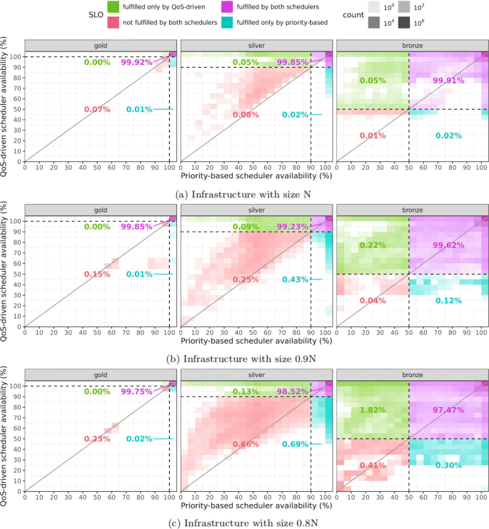

  

  QoS. QoS delivered to requests using QoS-driven and priority-based schedulers in different infrastructure sizes, and service classes

• 2 The bottom right quadrant (in blue) contains the availabilities of the requests that have their SLO satisfied by the priority-based scheduler, but not by the QoS-driven one.

• 3 The top left quadrant (in green) contains the availabilities of the requests that have their SLO satisfied by the QoS-driven scheduler, but do not by the priority one.

• 4 The bottom left quadrant (in red) contains the availabilities of the requests whose SLOs were violated by both schedulers.

The percentage associated with each quadrant represents the fraction of requests that fall in the quadrant. Thus, for each service class and infrastructure size, the SLO fulfillment for the priority-based scheduler can be computed by adding up the percentages associated with the bottom and top right quadrants (blue and purple), while that of the QoS-driven scheduler can be computed adding up the percentages associated with the top left and right quadrants (green and purple).

SLO fulfillment

The QoS-driven scheduler aims to maintain the QoS of the instances above their SLO and, in periods of high resource contention, deliver similar QoS to the instances of the same class competing for the same resources. This means that it is more prone to deliver higher QoS in general and, in periods of higher contention, it prioritizes fairness instead of SLO fulfillment. A decrease on the infrastructure size, increases the resource contention in the system, and makes the scheduling more challenging. As expected, as the infrastructure size is reduced, the SLO fulfillment in all quadrants in the heat maps shown in Fig. 6 diminishes. The SLO fulfillment achieved by the QoS-driven scheduler, compared with that provided by the priority-based one, is essentially the same for gold instances, in all infrastructure sizes, and for silver and bronze instances for the largest infrastructure. It is slightly lower for silver instances, and slightly higher for bronze instances, considering the other infrastructure sizes. The slight reduction on the SLO fulfillment in some cases, yield by the use of the QoS-driven scheduler, is explained by the fact that while trying to provide QoS closer to the SLO to all instances, this scheduler may increase the number of requests for which the QoS delivered is below the promised target. As discussed before, in periods of higher contention, the QoS-driven scheduler favors fairness within the service class, instead of SLO fulfillment. Nevertheless, this is more than compensated by the generally better QoS delivered, and fairer treatment to competing requests that are active at the same time. These benefits are thoroughly analyzed in the following.

QoS delivered to gold instances

In general, the availabilities of the gold requests are not different when the priority-based and QoS-driven schedulers are used. Regardless of the infrastructure size, almost all gold requests have their QoS target satisfied by both schedulers (99.75% in the worst case). The gold service class is the most QoS demanding class (100%) and, consequently, these requests are classified as the most important by both, the priority-based and the QoS-driven schedulers. For this reason, both schedulers, if needed, preempt all the instances of other classes (silver and bronze) for the benefit of gold instances. Therefore, it was expected that results for both schedulers were very similar.

The differences for this class occur due to the different packing mechanism used by the QoS-driven and the priority-based schedulers. This difference can be seen when we analyze the results of the workload sample 02. This workload has a peak of gold requests at day 5, when 150 gold requests are admitted at once, each one demanding around 31% of CPU of the largest host in Google’s infrastructure. This peak is very short and can be seen in Fig. 1 as a tiny green spike at day 5. At this moment, neither of the schedulers can allocate all the gold requests admitted, even after preempting silver and bronze instances. Although both schedulers decide to send all the silver and bronze instances of a host to the pending queue for the benefit of a gold instance, the scoring functions they use to assign instances to hosts are different: the QoS-driven scheduler considers the QoS metric, while the priority-based scheduler considers the priority and the arrival time. As a result, the actual allocation is not the same, and the gold instances can be allocated in different hosts depending on the scheduler used, causing different placements for these instances. Because of that, we see some gold instances in the blue quadrant (bottom right). It turns out that for workload sample 02, the priority-based scheduler was able to allocate a little more gold instances (0.02% in the worst case) than the QoS-driven one. We emphasize that this situation is particular to the workload used, and for other workloads the different placements for the gold instances could well lead to an opposite result.

QoS delivered to silver instances

Looking at the QoS delivered to the silver instances (central heat maps of Fig. 6), we see that, overall, the QoS-driven scheduler delivered higher availabilities. This result can be better visualized when we consider the identity line (diagonal) shown in these graphs. Every point that is above the identity line represents a request whose QoS delivered by the QoS-driven scheduler was higher than the QoS delivered by the priority-based one. We see that most of the points are concentrated above the identity line. This happens due to the fact that the two schedulers act differently during periods of resource contention. In particular, the QoS-driven scheduler is able to alternate which instances to run, irrespective of their classes, based simply on the current QoS delivered to the instances. In general, this leads the instances to achieve QoS closer to their targets. On the other hand, during resource contention periods, the priority-based scheduler does not alternate instances of the same class. Instead, it maintains some instances always running, and others always pending, based on their admission time. As a result: (i) many instances have very high QoS (shown as the darker squares in the vertical line of 100% availability in the blue quadrant), and (ii) many instances receive much lower QoS (shown by the more dispersed distribution in the green quadrant). In most of these cases, the QoS delivered to the instance was higher when the QoS-driven scheduler was used. These results are evidence of the effective use of the resources achieved by the QoS-driven scheduler that aims at maintaining the QoS of every instance as close as possible from its target.

By looking at the green and blue quadrants we see the different results achieved by the schedulers. In the blue quadrant we see the instances that violate their SLOs only when the QoS-driven scheduler is used. Most of the instances receive 100% of availability from the priority-based scheduler. The QoS delivered by the QoS-driven scheduler for these instances very seldom reached values below 45%, and was most of the time not very far from the target. On the other hand, when we analyse the cases when the QoS of silver instances are satisfied only by the QoS-driven scheduler (green quadrant), we see that the availabilities delivered by the priority-based scheduler were more dispersed, reaching very low availabilities. In cases when both schedulers violated the QoS target (red quadrant), the concentration of points above the identity line is clear. In this quadrant we see the cases where the QoS-driven scheduler offers low QoS to some instances. It is important to emphasize that for these instances, the priority-based scheduler has also delivered poor QoS. This is an indication that the QoS-driven scheduler offers very poor QoS only during periods of very high resource contention.

QoS delivered to bronze instances

Let us now analyze the QoS delivered to the bronze instances (plots on the right side of Fig. 6). For these instances, in general, the QoS-driven scheduler delivered higher availabilities. This fact is evidenced by considering the identity line in these graphs. We see that most of the points are concentrated above the identity line.

Since bronze instances are the less demanding in terms of QoS (50%), they can be left pending longer than the instances of other classes, without compromising the fulfillment of their SLOs. This means that the QoS-driven scheduler has more room to play with bronze instances. Basically, the scheduler alternates the bronze instances, stopping and starting them in a controlled way, to deliver a QoS that is close to their SLOs. Because of that, the QoS-driven scheduler increases the SLO fulfillment of the bronze instances in comparison with the priority-based scheduler, which prioritizes the instances that were admitted earlier.

In the green quadrant we see again many cases of poor QoS delivered by the priority-based scheduler, which does not alternate instances of the same class. While these instances are starving, there are probably others with very high QoS, far above the target. On the other hand, when only the priority-based scheduler satisfied the SLO (blue quadrant), the availabilities delivered by the QoS-driven scheduler were most of the time above 25%. Again, in cases when both schedulers violate the QoS target (red quadrant), the QoS-driven scheduler delivers poor QoS only in cases where the priority-based scheduler also delivers poor QoS, and almost always deliver a QoS that is higher.

Distribution of qoS deficits

In Fig. 7 we present the QoS deficits of the instances that had their SLOs violated. This metric is computed per instance, and is the difference between the SLO promised and the final availability delivered to the instance. In these plots, the wider is the width in the graph, the greater the quantity of points with that particular value. The 95% confidence interval of the QoS deficits measured for each particular scenario is also plotted in the graphs. Empty sub-graphs mean that no SLO violations occurred for those tests. The QoS deficits are presented individually for each workload sample, and grouped by service class.

Fig. 7

QoS deficit. QoS deficit of requests using QoS-driven and priority-based schedulers in different infrastructures size

Overall, we see larger QoS deficits when the priority-based scheduler is used, regardless of workload and infrastructure sizes. Moreover, there are more cases in which the QoS-driven scheduler accomplishes all the SLOs, while the priority-based scheduler does not. For both schedulers, the number of instances with QoS deficits increases as the infrastructure size decreases. Likewise, the extent of the deficits also increases as the infrastructure size decreases. However, in general, the QoS-driven scheduler managed to limit the QoS deficits to a smaller range and lower values.

When the infrastructure capacity is N (Fig. 7a), the QoS-driven scheduler managed to avoid QoS deficits for 4 workload samples: 03, 04, 08 and 09. These samples are among the ones with the highest peaks of non-gold requests (sample 08), or they have a good quantity of bronze instances (samples 03 and 04), or both (sample 09) — see Figs. 1 and 2. Based on how the infrastructure capacities were defined (described in Section 4.3), the workloads with huge peaks have extra resources, which allow both schedulers to allocate more requests over time. However, the QoS-driven scheduler has more flexibility to alternate which instances to run, leading to a more efficient use of the resources, when compared with the priority-based one.

The QoS-driven scheduler can still satisfy 100% of the SLOs for workload sample 03 when the size of the infrastructure is reduced to 0.9N (Fig. 7b), and to 0.8N (Fig. 7c). In this sample, the demand for gold instances is very flat over time. Besides, this sample has a good quantity of requests of the bronze class that can be preempted by the QoS-driven scheduler, and are not preempted by the priority-based one. By preempting these instances, the QoS-driven scheduler is able to accommodate all the load in a more efficient way.

Analyzing the QoS deficits shown in Fig. 7, sometimes we see deficits for the silver class, and not for the bronze class, when the QoS-driven scheduler is used (e.g. samples 05, 06 and 07, in all infrastructure sizes). These situations can give the wrong impression that the QoS-driven scheduler favored the bronze instances to the detriment of the silver ones. The first insight is that the scheduler could have taken the resources from the bronze instances to give to the silver instances. In reality, these samples have some peaks of demand of silver requests (see Figs. 1 and 2). In some of these peaks, both schedulers are not able to run all the silver instances anymore (even after preempting bronze instances). At these moments, the priority-based scheduler starts to enqueue new silver request arrivals. The QoS-driven scheduler acts differently: as soon as it realizes that there is not enough resources to run the silver demand, it starts to preempt the resources of some silver instances (in addition to bronze instances). From that moment on, the QoS-driven scheduler alternates which silver instances to run in such a way that the difference of current QoS delivered to these instances is minimized. During periods of high resource contention, all the resources were used to run instances associated to more important classes. After these periods, the QoS-driven scheduler can alternate which instances to run, while the priority-based one cannot preempt an instance for the benefit of another of the same class. This approach allows the QoS-driven scheduler to use the resources in a fairer way, choosing the right instances to run, in such a way that all bronze instances achieved their SLOs. Thus, the QoS-driven scheduler manages to fulfill all the SLOs of the bronze instances, not because it prioritizes these instances, but because it makes clever decisions to determine which requests should be running, and which should be left in the pending queue.

The penalty impact of SLA violations

The major public cloud providers (AWS and Azure) define SLAs whose penalties consider the level of QoS deficit experienced by customers. Thus, the penalties are not only defined based on the number of requests whose SLOs were violated, but also on the actual QoS delivered to these requests. For instance, AWS promises at least 99.99% of availability for its instances, in a monthly measurement. If an instance does not meet this QoS target, the customer will have a service credit according to the QoS received. In this case, AWS computes the service credits as a percentage of the total charges paid by the customer for the violating instance. When the availability provided is lower than 99.99%, but higher than 99.0%, the percentage of penalty is 10%. Then, this percentage increases to 30% for availabilities lower than 99.0%, and higher than 95.0%, and finally, it is set to 100%, when the availability provided is lower than 95.0%⁸.

Based on the AWS penalty model, we defined a model for assessing how the priority-based and the QoS-driven schedulers compare when we take into account the penalties that should be paid, corresponding to the requests whose SLOs they are unable to fulfill. We consider the same three levels of penalties for each service class provided: 10%, 30% and 100%. The penalties for the gold class follow the same rules of the AWS services. For the other classes (silver and bronze), we use similar rules, whose limits are proportionally set, taking into account the SLO that is promised to the class.

Let $\mathcal {A}_{j}(t)$ be the availability provided to a request j at time t when its execution completed. Table 2 presents the range of QoS for each class associated with the percentage of the credit to be paid by the provider when it delivers a QoS within the corresponding range.

Table 2 Percentage of the bonus credit to be paid to customers for each service class according to QoS delivered

In our model, the actual penalty to be paid is calculated taking into account both the duration of the violating request, as well as its resource demand. Let $D_{j}, D_{j} = \sigma _{i} - \mathcal {A}_{j}(t)$, be the QoS deficit experienced by a request j, d_j be its duration, i.e. the amount of time that j has run to be completed, and c_j be the amount of CPU requested by j, the CPU-hour deficit of j, $C^{-}_{j}$, is given by:

$$ C^{-}_{j} = D_{j} \cdot d_{j} \cdot c_{j}. $$

(10)

$C^{-}_{j}$ is the additional amount of CPU per time unit that j should have received to have its SLO satisfied. As the penalty for violating a request j, we define that the provider should pay $C^{-}_{j}$ incremented by a bonus, based on the QoS delivered to j, as presented in Table 2. Let b_j be the bonus credit to be paid by the provider related to j, then the penalty related to request j, P_j, is given by:

$$ P_{j} = C^{-}_{j} \cdot \left(1 + b_{j}\right). $$

(11)

In order to compare the penalties incurred to the provider using the two schedulers, we calculate P_j for each request j that had its SLO violated in the simulation tests. Figure 8 shows the increase on the penalty cost due by a provider using the priority-based scheduler when compared with the QoS-driven one. These values are calculated as the difference between the total penalty cost experienced when the priority-based scheduler is used and those experienced when using the QoS-driven one, divided by the total penalty cost experienced when the QoS-driven scheduler is used.

Fig. 8

Penalty. Increment on the penalty cost when using the priority-based scheduler in comparison to the QoS-driven scheduler

Our results show that the priority-based scheduler increases the total penalty cost incurred in comparison with those yield by the QoS-driven one, for all infrastructure sizes analyzed. When the infrastructure size is set to N, the total penalty cost obtained using the priority-based scheduler is almost twice that yield when the QoS-driven scheduler is used (91.5% higher), and the increase on the penalty cost is almost three times (193.7% higher), when the infrastructure capacity is set to 0.9N. Finally, for the lowest infrastructure size factor (0.8N), the increase on the penalty cost is very small (3%). In this case, the contention during critical periods is very high, leaving little margin for the different schedulers to maneuver. We recall that appropriate capacity planning and admission control should be in place to reduce the probability of such situation to happen.

Evaluation of the fairness

As discussed in the previous section, overall, the QoS-driven scheduler obtains QoS deficits that are smaller than those obtained by the priority-based one, for the same scenarios. However, it is important to evaluate the fairness delivered by the schedulers in shorter periods of time, considering only the requests that are active, instead of considering the whole simulation.

Given the variability of the workload demands over time, the system can experience different levels of resource contention in different points in time. For example, there is no resource contention in periods when all the admitted requests can be allocated, and receive 100% of availability. On the other hand, there is high resource contention when the provider cannot allocate the admitted requests in a way that all of them can achieve their QoS target. In general, smaller (resp. larger) infrastructures tend to result in a higher amount of periods with high (resp. low) level of resource contention. Nevertheless, periods of low and high resource contention can occur in infrastructures of the three sizes evaluated, depending on how the resource demand of the workload varies over time.

In periods when there is resource contention, the QoS-driven scheduler equally decreases the QoS of the instances within a class (delivering similar QoS to instances of the same class). For this reason, the QoS delivered to an instance in any point in time is directly related to the current level of resource contention. In order to evaluate the behavior of the QoS-driven scheduler according to the levels of resource contention, we split the execution of the simulations in shorter 10-min intervals. Each experiment test spanning 29 days was split in 4176 of such intervals.

Each interval was classified taking into account the resource contention level, as follows. Firstly, we identified the active requests of a particular interval. A request was active in an interval if it was admitted during this interval, or if it was admitted before this interval, and it was not terminated before the interval. We computed the availability of each active request according to Eq. 1. For the requests that were terminated during the particular interval, the time t considered while computing the availability was the moment that the request was terminated (i.e. this was the final availability of the request). In case of requests that were not terminated during the particular interval, the availability was computed considering the end of the interval.

Secondly, we used the results obtained by the priority-based scheduler to classify the level of resource contention as follows:

• 1 no contention: there are more resources than the demanded by all admitted requests. All requests of each class can be allocated during the interval and receive 100% of availability;

• 2 low contention: the priority-based scheduler can satisfy the SLO of all admitted requests. All requests of gold and silver classes receive 100% of availability, and bronze requests receive availability higher than its QoS target (50%), but below 100%;

• 3 medium contention: the priority-based scheduler cannot achieve the QoS target for bronze requests, but it delivers 100% of availability to requests of the gold and silver classes;

• 4 high contention: there are not enough resources for the priority-based scheduler to fulfill the SLO for all requests of gold and silver classes.

When a particular interval is classified as no contention, since the amount of resources is higher than the demand, both schedulers can allocate the admitted requests in a way that all of them receive 100% of availability. Thus, there is no difference between the schedulers in these intervals. For the other intervals, we compute three metrics based on the current availabilities of the active requests in a particular interval: (i) inequality of the availabilities, which give us an idea about the fairness of the scheduler. This is computed as the Gini coefficient of the availabilities delivered; the lower is the inequality of the availabilities of a particular class of requests, the fairer is the scheduling policy; (ii) minimum availability, which is the minimum availability of an active request in the particular interval. This metric indicates the worst case for the availability considering the active requests in the particular interval; and, (iii) current SLO fulfillment, which represents the partial SLO fulfillment of the active requests for each class in the particular interval. We note that the final availability of a request can be incremented or reduced by the time it is terminated.

Figure 9 presents the 95% confidence intervals for these three metrics, considering each level of resource contention, and service class.

Fig. 9

Fairness. Confidence intervals of the minimum availability, SLO fulfillment, and inequality of the availabilities of active requests, per service class, in 10-minute intervals with low, medium and high contention for resources

Looking at Fig. 9, we observe that there is no significant difference between the two schedulers in low contention intervals. We can highlight that the QoS-driven scheduler concentrates the minimal availabilities of bronze requests farther from the QoS target (50%), and the inequality for this class closer to 0. Nevertheless, both schedulers satisfy the SLO of all admitted requests, and there is no significant difference between their results.

In intervals classified as medium contention, the QoS-driven scheduler decreases the exceeding QoS from silver requests in order to improve the QoS delivered to bronze requests. This result can be visualized by the reduction of the minimum availability for silver requests, and the increment of this metric for bronze requests, when the QoS-driven scheduler is used, in comparison to when the priority-based one is used. By doing this, associated with the fact that the QoS-driven scheduler can also alternate the instances of the same class that are running, the QoS-driven scheduler increases significantly the current SLO fulfillment for the bronze class, without affecting the fulfillment of more important classes (gold and silver). It is also worth noting that the QoS-driven scheduler slightly increases the inequality of the availabilities for silver requests, while significantly reduces the inequality for bronze requests, comparing with values obtained when the priority-based scheduler is used. When the latter is used, all silver requests receive 100% of availability in these intervals, leading to a Gini coefficient of 0 (perfect equality). For this reason, when the QoS-driven scheduler preempts some silver requests for the benefit of other silver and bronze requests, it is introducing inequality for availabilities of the silver class. However, since this does not affect the fulfillment of silver requests, overall, it is not a problem in this scenario. The QoS-driven scheduler also reduces the inequality of availabilities for bronze requests. In this case, the QoS-driven scheduler can alternate the instances running in a way that the QoS delivered to bronze requests are more similar than the QoS delivered by the priority-based scheduler.

By analyzing the higher contention intervals, we note that the QoS-driven scheduler increases the minimum availability for silver and bronze requests. It happens because this scheduler can alternate the instances of the same class that are running, consequently, reducing the inequality of the availabilities within each class. However, this behavior was not enough to statistically improve the fulfillment for any class.

According to how the intervals were classified, all intervals where there is resource contention for at least one gold request is classified as higher contention (since a gold request needs to be always running in order to fulfill the 100% QoS target). However, as discussed in Section 5.1, the differences between the schedulers associated with gold requests occurred by chance.

In summary, medium contention intervals are the ones where the gains of the QoS-driven scheduler are more evident, in comparison with the priority-based one. However, the QoS-driven scheduler is fairer than the priority-based for silver and bronze requests even in periods of higher resource contention. We recall that the capacity planning and admission control activities performed in conjunction with the scheduling activity strive to avoid both over-provisioning and under-provisioning of the infrastructure. Thus, it is very important that the scheduler performs well in periods of moderate contention, which are the ones most likely to happen in a well configured system.

Conclusions

In this paper we present a new QoS-driven scheduling policy, which makes its decisions based on the QoS target and the actual QoS delivered for each request admitted. The QoS-driven scheduler aims at satisfying the SLAs of the requests, independently of their respective service classes, while promoting fairer treatment given to requests of the same class, even when the infrastructure is not enough to accommodate all of them. This goal is achieved by using a mechanism that allows preemptions of instances based on a QoS metric.

We evaluated this scheduling policy by comparing its performance against that of a state-of-the-practice priority-based scheduler, simulating the same realistic workloads on different infrastructure sizes. The simulation models were validated through measurement experiments based on an implementation of the QoS-driven scheduler for Kubernetes, and Kubernetes native priority-based scheduler.

The results show that, for extreme scenarios where the contention level is very high or very low (or even without contention), the QoS-driven scheduler has a behavior that is similar to the behavior of the priority-based one, with no significant difference in performance, in terms of QoS delivered. However, when contention level is moderate, the QoS-driven scheduler substantially increases the QoS delivered to requests with low QoS targets, by preempting instances whose QoS are exceeding their promised QoS. We note that the capacity planning and admission control mechanisms that operate in conjunction with the scheduler will try to avoid both over-provisioning of the infrastructure — to keep costs as low as possible —, as well as under-provisioning — to keep QoS at adequate levels. Thus, a scheduler that performs well in periods of medium contention is very useful. In this moderate scenario, pursued by providers, bronze instances show a considerable increase on the average of the minimum availability delivered (from 7% to 90%), as well as on the mean QoS fulfillment gain. This comes with a tiny reduction on the availability of silver instances, which does not compromise the QoS fulfillment of the silver class.

Moreover, considering the periods of time when not all requests can get the promised QoS, a scheduler that tries to minimize the QoS deficit and diminish the variability of the QoS delivered to requests of the same class is in line with the way that the major public cloud providers define their SLAs. For instance, both AWS⁹ and Azure¹⁰ have SLAs whose penalties vary in a non-linear way with the QoS deficit experienced by customers — larger deficits lead to increasingly larger penalties. Evaluating the penalties incurred to the providers due to SLA breaches when the contention level is moderate, the use of the priority-based scheduler leads to a total penalty cost that is about 193% higher, compared with the total penalty cost due when using the QoS-driven scheduler.

References

Marshall P, Keahey K, Freeman T. Improving utilization of infrastructure clouds. In: Proceedings of the 2011 11th IEEE/ACM International Symposium on Cluster, Cloud and Grid Computing CCGRID ’11. Washington: IEEE Computer Society: 2011. p. 205–14.
Amazon EC2 - Instances pricing. 2019. https://aws.amazon.com/ec2/pricing/. Accessed 28 Nov 2019.
Google Compute Engine - Preemptible Instances. 2019. https://cloud.google.com/compute/docs/instances/preemptible. Accessed 15 Dec 2019.
Carvalho M, Cirne W, Brasileiro F, Wilkes J. Long-term slos for reclaimed cloud computing resources. In: Proceedings of the ACM Symposium on Cloud Computing SOCC ’14. New York: ACM: 2014. p. 1–13.
Carvalho M, Menasce D, Brasileiro F. Prediction-based admission control for iaas clouds with multiple service classes. In: Proceedings of the 2015 IEEE 7th International Conference on Cloud Computing Technology and Science (CloudCom) CLOUDCOM ’15. Washington: IEEE Computer Society: 2015. p. 82–90.
Xu J, Zhu C. Optimal pricing and capacity planning of a new economy cloud computing service class. In: 2015 International Conference on Cloud and Autonomic Computing. Washington: IEEE Computer Society: 2015. p. 149–57.
Cirne W, Frachtenberg E. Web-scale job scheduling. Lecture Notes in Computer Science. 2013; 7698:1–15.
Vavilapalli VK, Murthy AC, Douglas C, Agarwal S, Konar M, Evans R, Graves T, Lowe J, Shah H, Seth S, Saha B, Curino C, O’Malley O, Radia S, Reed B, Baldeschwieler E. Apache hadoop yarn: Yet another resource negotiator. In: Proceedings of the 4th Annual Symposium on Cloud Computing SOCC ’13. New York: ACM: 2013. p. 1–16.
Verma A, Pedrosa L, Korupolu M, Oppenheimer D, Tune E, Wilkes J. Large-scale cluster management at google with borg. In: Proceedings of the Tenth European Conference on Computer Systems EuroSys ’15. New York: ACM: 2015. p. 1–17.
Schwarzkopf M, Konwinski A, Abd-El-Malek M, Wilkes J. Omega: Flexible, scalable schedulers for large compute clusters. In: Proceedings of the 8th ACM European Conference on Computer Systems EuroSys ’13. New York: ACM: 2013. p. 351–64.
Karanasos K, Rao S, Curino C, Douglas C, Chaliparambil K, Fumarola GM, Heddaya S, Ramakrishnan R, Sakalanaga S. Mercury: Hybrid centralized and distributed scheduling in large shared clusters. In: Proceedings of the 2015 USENIX Conference on Usenix Annual Technical Conference USENIX ATC ’15. Berkeley: USENIX Association: 2015. p. 485–97.
Boutin E, Ekanayake J, Lin W, Shi B, Zhou J, Qian Z, Wu M, Zhou L. Apollo: Scalable and coordinated scheduling for cloud-scale computing. In: Proceedings of the 11th USENIX Conference on Operating Systems Design and Implementation OSDI’14. Berkeley: USENIX Association: 2014. p. 285–300.
Delimitrou C, Sanchez D, Kozyrakis C. Tarcil: Reconciling scheduling speed and quality in large shared clusters. In: Proceedings of the Sixth ACM Symposium on Cloud Computing SoCC ’15. New York: ACM: 2015. p. 97–110.
Burns B, Grant B, Oppenheimer D, Brewer E, Wilkes J. Borg, omega, and kubernetes. Commun ACM. 2016; 59(5):50–7.
Wilkes J. More Google cluster data. Google research blog. 2011. https://ai.googleblog.com/2011/11/more-google-cluster-data.html.
Reiss C, Tumanov A, Ganger GR, Katz RH, Kozuch MA. Heterogeneity and dynamicity of clouds at scale: Google trace analysis. In: Proceedings of the Third ACM Symposium on Cloud Computing SoCC ’12. New York: ACM: 2012. p. 1–13.
Curino C, Difallah DE, Douglas C, Krishnan S, Ramakrishnan R, Rao S. Reservation-based scheduling: If you’re late don’t blame us!. In: Proceedings of the ACM Symposium on Cloud Computing SOCC ’14. New York: ACM: 2014. p. 1–14.
Dubey S, Agrawal S. Qos driven task scheduling in cloud computing. Int. J. Comput. Appl. Technol. Res. 2013; 2(5):595–600.
Wu X, Deng M, Zhang R, Zeng B, Zhou S. A task scheduling algorithm based on qos-driven in cloud computing. Procedia Computer Sci. 2013; 17:1162–9.
Delimitrou C, Kozyrakis C. Quasar: resource-efficient and qos-aware cluster management. ACM SIGPLAN Notices. 2014; 49(4):127–44.
Goiri I, Julia F, Nou R, Berral JL, Guitart J, Torres J. Energy-aware scheduling in virtualized datacenters. In: Proceedings of the 2010 IEEE International Conference on Cluster Computing CLUSTER ’10. Washington: IEEE Computer Society: 2010. p. 58–67.
Kong X, Lin C, Jiang Y, Yan W, Chu X. Efficient dynamic task scheduling in virtualized data centers with fuzzy prediction. J Netw Comput Appl. 2011; 34(4):1068–77.
Delimitrou C, Kozyrakis C. Paragon: Qos-aware scheduling for heterogeneous datacenters. SIGPLAN Not. 2013; 48(4):77–88.
Ousterhout K, Wendell P, Zaharia M, Stoica I. Sparrow: Distributed, low latency scheduling. In: Proceedings of the Twenty-Fourth ACM Symposium on Operating Systems Principles SOSP ’13. New York: ACM: 2013. p. 69–84.
Shahrad M, Wentzlaff D. Availability knob: Flexible user-defined availability in the cloud. In: Proceedings of the Seventh ACM Symposium on Cloud Computing SoCC ’16. New York: ACM: 2016. p. 42–56.
He X, Sun X, Von Laszewski G. Qos guided min-min heuristic for grid task scheduling. J Comput Sci Technol. 2003; 18(4):442–51.
Silva G, Lopes R, Brasileiro F, Carvalho M, Morais F, Mafra J, Turull D. Fair scheduling in cloud infrastructures with multiple service classes (in Portuguese). In: Proceedings of the 37th Brazilian Symposium on Computer Networks and Distributed Systems. Porto Alegre: SBC: 2019. p. 636–49. https://sol.sbc.org.br/index.php/sbrc/article/view/7392.
Pan W, Rowe J, Barlaoura G. Records in the cloud (ric) user survey report. Tech Rep Univ British Columbia. 2013. doi:10.14288/1.0075820.
Liu CL, Layland JW. Scheduling algorithms for multiprogramming in a hard-real-time environment. Journal of the ACM (JACM). 1973; 20(1):46–61.
Lopes RV, Menascé D. A taxonomy of job scheduling on distributed computing systems. IEEE Trans Parallel Distrib Syst. 2016; 27(12):3412–28.
Reiss C, Wilkes J, Hellerstein JL. Google cluster-usage traces: format + schema. Technical report, Google Inc. 2014.
Carvalho M, Menascé DA, Brasileiro F. Capacity planning for iaas cloud providers offering multiple service classes. Futur Gener Comput Syst. 2017; 77:97–111.
Tirmazi M, Barker A, Deng N, Haque ME, Qin ZG, Hand S, Harchol-Balter M, Wilkes J. Borg: the next generation. In: EuroSys’20. Heraklion: 2020. p. 1–14.
Bellu LG, Liberati P. Inequality Analysis: The Gini Index. Food Agric Organ U N FAO. 2006; 40:6–9.
Acknowledgments
Not applicable.
Funding
This work was funded by the Innovation Center, Ericsson Telecomunicações S.A., Brazil, and by EMBRAPII-CEEI.
Author information
Authors and Affiliations
Contributions
GFS, FB, RL, MC, and DT jointly came up with the concept of QoS-driven scheduling. GFS developed the simulation model and, together with FM, developed the proof-of-concept implementation. All authors participated in the analysis of the experiment results. GFS, FB and RL drafted most of the manuscript. MC, FM and DT revised the manuscript in several interactions. All authors read and approved the final manuscript.
Corresponding author
Ethics declarations
Competing interests
The authors declare that they have no competing interests.
Additional information
Publisher’s Note
Springer Nature remains neutral with regard to jurisdictional claims in published maps and institutional affiliations.
Rights and permissions
Open Access This article is licensed under a Creative Commons Attribution 4.0 International License, which permits use, sharing, adaptation, distribution and reproduction in any medium or format, as long as you give appropriate credit to the original author(s) and the source, provide a link to the Creative Commons licence, and indicate if changes were made. The images or other third party material in this article are included in the article’s Creative Commons licence, unless indicated otherwise in a credit line to the material. If material is not included in the article’s Creative Commons licence and your intended use is not permitted by statutory regulation or exceeds the permitted use, you will need to obtain permission directly from the copyright holder. To view a copy of this licence, visit http://creativecommons.org/licenses/by/4.0/.
About this article
Cite this article
da Silva, G.F., Brasileiro, F., Lopes, R. et al. QoS-driven scheduling in the cloud. J Internet Serv Appl 11, 9 (2020). https://doi.org/10.1186/s13174-020-00129-0
Published:
DOI: https://doi.org/10.1186/s13174-020-00129-0