An optimization-based approach for efficient network monitoring using in-band network telemetry

Abstract

In recent years, as a result of the proliferation of non-elastic services and the adoption of novel paradigms, monitoring networks with high level of detail is becoming crucial to correctly identify and characterize situations related to faults, performance, and security. In-band Network Telemetry (INT) emerges in this context as a promising approach to meet this demand, enabling production packets to directly report their experience inside a network. This type of telemetry enables unprecedented monitoring accuracy and precision, but leads to performance degradation if applied indiscriminately using all network traffic. One alternative to avoid this situation is to orchestrate telemetry tasks and use only a portion of traffic to monitor the network via INT. The general problem, in this context, consists in assigning subsets of traffic to carry out INT and provide full monitoring coverage while minimizing the overhead. In this paper, we introduce and formalize two variations of the In-band Network Telemetry Orchestration (INTO) problem, prove that both are NP-Complete, and propose polynomial computing time heuristics to solve them. In our evaluation using real WAN topologies, we observe that the heuristics produce solutions close to optimal to any network in under one second, networks can be covered assigning a linear number of flows in relation to the number of interfaces in them, and that it is possible to minimize telemetry load to one interface per flow in most networks.

1 Introduction

Monitoring is an essential component of network operation and management tasks. In recent years, monitoring networks with high level of detail (e.g., per-packet hop-by-hop delays, instantaneous queue size) is becoming crucial to correctly identify and characterize network events related to faults, performance, and security. This new requirement can be attributed, in part, to the proliferation of non-elastic services (e.g., telesurgery, virtual reality video streaming) that demand timely, fine-grained and accurate monitoring to identify and quickly react to sources of substantial delay and jitter [1]. The adoption of novel technologies and paradigms, such as network virtualization and software-defined networking (SDN), also demands more detailed information about network state and behavior to allow more informed decisions (e.g., routing, buffer sizes).

Traditional tools fall short at correctly dealing with the new monitoring demands or at providing the necessary level of detail while keeping reasonable overheads since these tools were not designed with those requirements in mind. Recent efforts have explored new monitoring opportunities that arise in the context of SDN to provide better visibility into the network. NetSight [2], Everflow [3] and Stroboscope [4] considered the use of packet mirroring to create packet histories that indicate paths and estimate hop-by-hop delays. Payless [5] and AdaptiveSampling [6] proposed dynamically adjusting the frequency of flow record polling from OpenFlow switches to manage overheads.

All of these investigations have important limitations. First, when several switches in the path of a packet mirror it, the copies need to be transmitted through the network. Thus, the monitoring data is considerable and can become a significant source of degradation depending on the network size and level of activity. Second, these approaches have limited accuracy and level of detail. For example, in the case of Payless and AdaptiveSampling, even if the polling frequency is very high, the level of detail of the data would not be sufficient to detect situations such as intermittent congestion events in the order of microseconds. Finally, all these studies have limited their scope to traditional SDN, and do not consider recent advances in data plane programmability [7–9].

More recently, a new monitoring concept has been proposed: In-band Network Telemetry (INT) [10–12]. It makes use of new capabilities of emerging programmable switches [7, 9, 13] to encapsulate processing metadata information (e.g., queue occupancy, processing time, policy rules) into “production traffic” packets (i.e., packets originated at the application layer). This information is accumulated in a packet along its path and, at some point in the network, extracted and reported to a monitoring control entity. The collection of this information has the objective of continuously identifying state, behavior, and performance of a network as perceived by its traffic.

INT may be applied to produce monitoring data with an unparalleled level of accuracy and detail [11, 14]. That is because instead of relying on active probes, which may be subject to forwarding and routing behaviors different from those of the traffic of interest, the production packets themselves can be used to probe the network. Moreover, for metadata that changes over time (e.g., queue occupancy), measurements can be made precisely during the instants when certain packets of interest are being processed at a device. This level of detail and accuracy makes possible to detect and pinpoint network events that were previously imperceptible, such as microsecond congestion.

Although INT brings new opportunities regarding accuracy and level of detail, to be able to use it in practice, there is the need to understand the trade-offs between quality and costs involved in employing it. Executing this type of telemetry involves modifying production packets traversing the network, which may significantly degrade the performance of end-user applications. In a previous work [15], we have made an initial effort to identify and characterize the limitations associated with it and the factors that impact performance. The amount of metadata that may be inserted into a packet is restricted by its original size and the network maximum transmission unit (MTU). The level of degradation is a consequence of factors such as in-flight packet size variation, sharing level of device and link resources between application and monitoring data, and the processing demand imposed by metadata report packets. We argue that these factors need to be carefully considered when monitoring networks using in-band network telemetry.

In this work, we introduce the In-band Network Telemetry Orchestration (INTO) problem, which is focused on optimizing the use of network resources for INT. Our ultimate goal is to minimize overheads while obtaining high-quality monitoring data. We formalize two variations of the INTO problem as mathematical programming models and prove that both are NP-Complete problems. We also introduce heuristic algorithms designed to generate high-quality polynomial computing time solutions to the variations of the INTO problem. We evaluate the quality and costs of the proposed strategies under realistic scenarios, and compare their results to allow identifying what types of networks they are better suited to monitor.

The remainder of the paper is organized as follows. We start, in Section 2, by briefly reviewing data plane programmability and INT concepts. We also revisit the challenges and degradation factors associated with the use of INT. In Section 3, we formally define the In-band Network Telemetry Orchestration (INTO) problem and propose mathematical programming models to solve the two optimization variations of it. In Section 4, we introduce the proposed heuristic algorithms. In Section 5, we evaluate the proposed mathematical programming models and heuristic algorithms and compare the two variations of the problem. In Section 6, we discuss the related work. And in Section 7 we present our concluding remarks.

2 Background

Recently, data plane programmability has emerged as a novel concept for evolving the software-defined networking paradigm [7]. It allows network operators to specify how the forwarding devices in a network should parse packet headers (standard or custom) and process packets using a domain-specific programming language such as P4 [8]. This new level of flexibility decouples the development of network protocols and the design of switching chips [8, 10] thus enabling quicker deployment of new services.

One example of concept service that has been facilitated by programmable data planes is In-band Network Telemetry (INT) [10, 11]. It makes use of the opportunity to define custom headers, tables, and processing logic to insert information about the network state (e.g., link utilization, switch buffer occupancy, hop-by-hop delays) into “production traffic” packets [11]. This telemetry data is subsequently and transparently extracted by a switch and reported to a monitoring sink/analyzer, while the packets with their original content are delivered to the recipient hosts [12].

INT provides a way for monitoring networks and services with high accuracy and level of detail [16]. Despite these benefits, because it uses production traffic, it is important to consider constraints imposed by the traffic and potential impacting factors to perform it effectively and efficiently. The key constraint of INT is that packets cannot exceed the network MTU. Therefore, the length of the telemetry data that can be embedded into a packet is limited by the difference between its original size and the MTU. The smaller the packet, the larger its telemetry capacity (i.e., the number of metadata items it can transport). All orchestration strategies have to comply with this constraint, which may limit the number of interfaces that can be monitored in a network. Next, we present and discuss the main factors that may lead to network performance degradation, as identified in our previous work [15].

• (a) Embedding telemetry data into packets causes their size to increase along their paths. Making packets increase in size may cause jitter in their transmission. Jitter may degrade the QoS of many applications, specially of non-elastic ones (e.g., VoIP, virtual reality video streaming).

• (b) Packet forwarding devices have limited processing capacity. The generation of telemetry report packets uses this capacity, thus, forwarding too many reports may saturate devices.

• (c) Monitoring sinks and analyzers have limited processing capacity. Receiving too many report packets and too many telemetry data may saturate these machines, which could impair their capacity to properly monitor the network.

• (d) Network links have limited bandwidth. The telemetry data transported in production packets uses the bandwidth of links in the network. If too much data is inserted into packets and reported to sinks, the growth in data volume may saturate links and devices.

The level of impact of the factors mentioned above is intrinsically related to the assignment of INT tasks to the traffic in the network. Figure 1 illustrates the “full” assignment of telemetry tasks, which is a straightforward method to carry out INT. The network in Fig. 1 is composed of five forwarding devices and has endpoints to four other networks (e₁−e₄). Moreover, there are four packet flows of the same traffic type: f₁:e₁⇔e₄, f₂:e₁⇔e₂, f₃:e₂⇔e₃, and f₄:e₃⇔e₄. The full assignment represents a scenario where every flow in the network would collect (and transport) metadata items from all device interfaces in its path. For example, the packets of flow f₄ collect information about interfaces J, K, M, and N, as it is indicated by the orange circles in the figure.

Fig. 1

Example of full assignment

The full assignment has significant drawbacks. First, it is not aware of telemetry demands and capacities. For example, consider the case where interfaces J, K, M, and N had each four telemetry items to be collected, and the telemetry capacity of flow f₄ was 12 items (according to the typical size of packets). In this case, the full assignment would be unfeasible, because by the time packets coming from e₃ arrived at interface N they would not have enough space to collect the four items from it. Therefore, the full assignment does not guarantee that, in practice, flows will cover all interfaces in their paths.

Second, all flows are subject to the performance degradation factors discussed previously in this section, as the full assignment is not selective in its choices. Third, all telemetry supporting tasks (i.e., telemetry header creation and extraction, report packet generation and transmission) tend to be executed by edge devices, increasing their probability of being saturated. Fourth, device interfaces are often monitored by multiple flows, each of them collecting the instantaneous value of same metadata items. Previous work [11, 14] has shown that it is possible to obtain instantaneous metadata with microsecond granularity using only one out of all flows traversing an interface or forwarding device. Furthermore, since all flows are of the same traffic type, behavioral and performance metadata (e.g., forwarding rules, queue delay) is expected to be similar. Finally, in this assignment the INT overhead is highly influenced by the level of activity in the network (i.e., the number of flows). Thus, an increase in network activity may inadvertently saturate its links and devices.

In summary, we advocate that network monitoring through INT requires some sort of task orchestration to be viable in practice. In the next sections, we present our proposed solution, starting, next, with the formalization of INT orchestration as an optimization problem.

3 In-band network telemetry orchestration optimization

In general terms, the problem under study – entitled In-Band Network Telemetry Orchestration (INTO) problem – consists in monitoring network device interfaces effectively (covering all monitoring demands) and efficiently (minimizing resource consumption and processing overheads). We start the problem definition by formally describing the input and output of our optimization models. For convenience, Table 1 presents the complete notation used in the formulation.

Table 1 Summary of symbols

The INTO problem considers a physical network infrastructure G=(D, I) and a set of network flows F. Set D in network G represents the programmable forwarding devices D={1,2,...,|D|}. Each device d∈D has a set of network interfaces that are connected to other devices in the network. We denote the interface of a device d_a that is connected to a device d_b by the tuple (d_a,d_b). Similarly, the interface of d_b that is connected to d_a is denoted by (d_b,d_a). The set of all device interfaces in the network is denoted by I. For each interface i∈I, there is an associated monitoring demand, a fixed number of telemetry items $\delta (i) \in \mathbb {N}^{+}$ that need to be collected periodically by flows in F. The interface telemetry demands are determined by monitoring policies, which are influenced by, for example, the level of activity of each interface or a previously detected event of interest.

The set F represents a group of aggregate packet flows of the same traffic type that are active in the network. In the case where the operator wants to monitor different types of traffic (e.g., scientific computing, video streaming, VoIP), a separate problem instance could be created for each one with their respective flows. This is done because the metadata values observed by a flow may be different from the values observed by other flows, specially for performance-related metadata [17]. For example, if a network prioritizes forwarding VoIP traffic in detriment of Web traffic, the queueing time observed by packets of each type may be different. Thus, if an operator wants to obtain metadata that is highly consistent with a specific type of traffic, the best approach to guarantee this would be to create a problem instance for each type of traffic. We note that the INTO problem definition and our solutions do not preclude operators from treating all traffic as a single type. Creating separate instances is therefore a recommendation for the obtention of more consistent monitoring data.

Each flow f∈F has two endpoints (ingress and egress) and is routed within the network infrastructure G using a single path. We denote the path ρ(f) of a specific flow f as a list of interfaces through which its packets are forwarded. For example, a network flow f from endpoint s to t routed through forwarding devices 1, 3, and 4 has ρ(f)=(1,s),(1,3),(3,1),(3,4),(4,3),(4,t). The first forwarding device interface visited is that of device 1 connected to the ingress endpoint (s), and the last is that of device 4 connected to the egress endpoint (t). Associated with each flow f is also a telemetry capacity $\kappa (f) \in \mathbb {N}^{+}$, which is the maximum number of items each packet of the flow may transport. The capacity of the flows is determined by factors such as forwarding protocols (e.g., IPv4, IPv6, NSH [18]), packet sizes, and network monitoring policies. The telemetry capacity may differ from packet to packet in a single flow, but we expect that the distribution of sizes is stable to be estimated with historic data. The capacity of (aggregate) flows can be defined according to percentile values of the distribution of sizes in order to guarantee that most (e.g., 90%) of the packets will have enough space to collect the metadata of the interfaces they are assigned to cover.

Given the problem input, an INTO optimization model will try to find a feasible assignment Φ:I→F that optimizes a specific objective function, where Φ(i)=f indicates that flow f∈F should cover interface i∈I. A feasible assignment is one where (i) each interface is covered by exactly one of all flows in F that pass through it and (ii) no flow f∈F is assigned to cover more interfaces than its capacity allows, i.e., the sum of demands from all interfaces covered by a flow does not exceed its capacity.

We highlight two important design decisions in our models. First, assignment function Φ does not enable partitioning the demand of an interface across multiple flows. We chose this type of assignment because some of the items to be collected on an interface are interdependent. For example, when collecting the transmission utilization it is also necessary to collect the ID of the respective interface. Enabling items to be balanced in different flows would require adjusting the models to assign flows to cover individual items instead of interfaces and introducing additional restrictions to force certain assignments in order to satisfy interdependency requirements. At this point, it is not clear that enabling such granularity in assignment would bring advantages enough to counter the complexity that would be introduced to the models, but we do consider further investigating this possibility in a future work.

Second, our model assigns a single aggregate flow per interface. We observe that, in some cases, it may be useful to introduce limited assignment redundancy. For example, to guarantee coverage and reduce the number of necessary configuration updates in a scenario of highly frequent changes in the set of flows. In our work, this redundancy is implicitly achieved through the employment of the “grain” of aggregate flows traversing a network core, which tend to present small and few changes over time. We leave exploring alternative options for both of these design decisions for future work.

Considering the key traffic constraint and main performance influencing factors discussed in Section 2, we define two optimization problems, namely, INTO Concentrate and INTO Balance. Next, we present the two optimization problems. For each problem we describe its objective function, propose an optimization model to solve it and prove that it is an NP-Complete problem.

3.1 INTO concentrate optimization problem

The number of flows participating in monitoring the network via INT dictates the number of telemetry report packets generated periodically since a report is sent for each packet of each telemetry-active flow. As previously discussed, creating too many report packets may saturate the forwarding devices that are tasked with their generation and the machines tasked with their analysis. Therefore, one possible optimization goal is minimizing the number of telemetry-active flows. That is the objective of the INTO Concentrate problem.

3.1.1 Example assignment

Figure 2 shows an example “Concentrated assignment”, i.e., an assignment that uses the optimal number of telemetry-active flows for our running example previously presented in Fig. 1 of Section 2. The example assignment shows that it is possible to cover all device interfaces using only three out of the four flows in the network. Flows f₁ and f₃ are assigned to cover six interfaces each, {A, B, E, H, L, N} and {J, I, G, F, C, D}. Flow f₄ is assigned to monitor the remaining two uncovered interfaces K and M, while flow f₂ is not assigned to cover any interface.

Fig. 2

Concentrated assignment example

3.1.2 Optimization model

The proposed optimization model to solve INTO Concentrate is presented next as an integer linear program. Variable x_{i, f} indicates whether flow f should cover interface i∈I. The values of all variables x_i,f define the assignment function Φ, i.e., x_{i, f}=1→Φ(i)=f. Variable y_f indicates whether flow f is a telemetry-active flow (i.e., if it covers at least one interface). This second set of variables is necessary to compute the objective function of the problem, the number of telemetry-active flows (Eq. 1).

$$\begin{array}{*{20}l} \text{min} & \Phi_{c} = \sum\limits_{f \in F} y_{f} \end{array} $$

(1)

$$\begin{array}{*{20}l} \text{s.t.} & \sum\limits_{f \in F} x_{i, f} = 1, & \forall i \in I, \delta(i) > 0 \end{array} $$

(2)

$$\begin{array}{*{20}l} & \sum\limits_{i \in \rho(f)} x_{i,f} \cdot \delta(i) \leq y_{f} \cdot \kappa(f), & \forall f \in F \end{array} $$

(3)

$$\begin{array}{*{20}l} & x_{i,f} \in \{0, 1\}, & \forall i \in I, \forall f \in F \end{array} $$

(4)

$$\begin{array}{*{20}l} & y_{f} \in \{0, 1\}, & \forall f \in F \end{array} $$

(5)

The objective function (Eq. 1) defines the minimization of the number of telemetry-active flows by the sum of the y variables. Constraint set in Eq. 2 ensures that all interfaces i∈I with positive demand are covered by some flow f∈F. Constraint set in Eq. 3 bounds the number of telemetry items each flow f∈F can be assigned to collect and transport according to its capacity κ(f). Equation 3 also activates y_f when any telemetry item is assigned to flow f∈F. Constraint sets in Eqs. 4 and 5 define the domains of variables x_i,f and y_f, which are binary.

3.1.3 Proof of NP-completeness

We will now prove that the decision version of the INTO Concentrate problem is an NP-Complete problem. Given a network infrastructure G=(D, I), the set of network flows F, and an integer number n; the goal of the decision version of the problem is to determine whether there exists a feasible assignment Φ where no more than n flows are used to transport telemetry items.

Lemma 1

INTO Concentrate belongs to the class NP.

We prove that the decision version of the INTO Concentrate problem is in NP by way of a verifier. Given any assignment Φ:I→F, the verifier needs to check three conditions. First, that the number of telemetry-active flows is indeed at most n (in $\mathcal {O}(|F|)$ time). Second, that every interface is covered (in $\mathcal {O}(|I|)$ time). Third, that no flow collects more telemetry items than its capacity (in $\mathcal {O}(|I||F|)$). For a yes instance (G, F, n), the certificate is any feasible assignment using n flows in F; the verifier will accept such an assignment. For a no instance (G, F, n), it is clear that no assignment using n flows of F will be accepted by the verifier as a feasible assignment.

Lemma 2

Any Bin Packing problem instance can be reduced in polynomial time to an instance of the INTO Concentrate Decision problem.

An instance of the Bin Packing Problem (BPP), which is a classical NP-Complete problem [19], comprises a set A of items, a size s_a for each item a∈A, a positive integer bin capacity C, and a positive integer n. The decision version of the BPP asks if its possible to pack all items into n bins, i.e., if there is a partition of A into n disjoint sets (B₁,B₂,...,B_n) such that the sum of sizes of the items in each subset is at most C. The INTO Concentrate problem is a generalization of the BPP where bins may have different capacities and each item may only be put on a specific subset of all bins. We reduce any instance of the BPP to an instance of the INTO Concentrate problem using the following procedure. The reduction has polynomial time complexity $\mathcal {O}(n|A|)$.

• 1. An infrastructure G is created with |A| forwarding devices and two endpoints e_s and e_t. See example in Fig. 3, device numbers are shown in bold. The devices are connected in line, i.e., device a∈A is connected to device b=a+1,b∈A. Devices a=1 and a=|A| are also connected to endpoints e_s and e_t, respectively. The interface of each device a=1,2,...,|A| that is connected to the next device (or to endpoint e_t in the case of device a=|A|) has telemetry demand equal to s_a, while the other interface has no telemetry demand. The interface demands are shown in italics in the figure.

  Fig. 3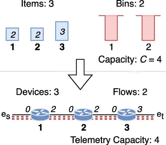

  

  Example BPP reduction to INTO Concentrate. A BPP instance with |A|=3 items, bin capacity C=4, and number of bins n=2 is reduced to an INTO Concentrate instance with 3 forwarding devices and 2 flows with telemetry capacity equal to 4 items

• 2. Next, n flows (B₁,B₂,...,B_n) are created. Each flow has endpoints e_s and e_t and is routed through a path comprising all forwarding device interfaces in G, i.e., ρ(B_i)=(1,e_s),(1,2),(2,1),...,(|A|,e_t),i=1,2,...,n. The telemetry capacity of all flows is C.

Theorem 1

The INTO Concentrate decision problem is NP-Complete.

Proof

By the instance reduction presented, if a BPP instance has a solution using n bins, then the INTO Concentrate problem has a solution using n flows. Consider that each item a of size s_a packed into a bin B_i corresponds to the coverage of the interface of device a with positive telemetry demand by flow B_i. Conversely, if the INTO Concentrate problem has a solution using n flows, then the corresponding BPP instance has a solution using n bins. Covering the positive demand interface of device a with flow B_i corresponds to packing an item of size s_a into bin B_i. Lemmas 1 and 2 complete the proof. □

3.2 INTO balance optimization problem

The number of telemetry items to be collected by each flow determines how much a packet will grow in size during its forwarding inside the network. If too many telemetry items are concentrated into one flow, the links through which its packets are forwarded may be saturated by significant growth in data volume. Consequently, another optimization goal would be to balance the telemetry demands among as many flows as possible. This assignment strategy would minimize the probability of saturating any single link because the variation in data volume becomes minimal for each flow. The INTO Balance objective is to minimize the maximum number of telemetry items transported (i.e., telemetry load) by any single flow.

3.2.1 Example assignment

Figure 4 illustrates a possible Balanced assignment, i.e., one that achieves the optimal telemetry load balance, for the example scenario previously presented in Figs. 1 and 2. This example assignment shows that it is possible to cover all device interfaces in the network while assigning no more than four interfaces (i.e., collecting 4×4=16 items) per telemetry-active flow. The optimal load balance value is determined by three factors: (i) the maximum telemetry demand per single interface, (ii) the fraction between the sum of all interface demands and the number of flows, and (iii) the different flow to interface assignment options. In the example, all interfaces have equal demand of four items. The total sum of demands 14interfaces×4 items=56 items divided by the four flows equals 14 items per flow. Since a flow must collect all (or none) of the items of an interface, the optimal load balance is found when two flows are assigned to collect 16 items each (i.e., cover four interfaces) and the other two are assigned to collect 12 items (i.e., cover three interfaces). The assignment shown in Fig. 4 follows this distribution. Flows f₂ and f₃ are assigned to four interfaces each, {A, B, D, F} and {C, G, I, J}. Likewise, f₁ and f₄ are assigned to three interfaces each, {E, H, L} and {K, M, N}.

Fig. 4

Balanced assignment example

3.2.2 Optimization model

Next, we present the integer linear program to solve the INTO Balance optimization problem. Variable x_{i, f} indicates whether flow f∈F should cover interface i ∈ I. As was the case with the Concentrate model, the values of variables x_{i, f} define the assignment function Φ, i.e., x_{i, f}=1→Φ(i)=f. Variable k indicates the maximum number of telemetry items assigned to be collected and transported by a single flow.

$$\begin{array}{*{20}l} \text{min} & \Phi_{b} = k \end{array} $$

(6)

$$\begin{array}{*{20}l} \text{s.t.} & \sum\limits_{f \in F} x_{i, f} = 1, & \forall i \in I, \delta(i) > 0 \end{array} $$

(7)

$$\begin{array}{*{20}l} & \sum\limits_{i \in \rho(f)} x_{i,f} \cdot \delta(i) \leq \kappa(f), & \forall f \in F \end{array} $$

(8)

$$\begin{array}{*{20}l} & \sum\limits_{i \in \rho(f)} x_{i,f} \cdot \delta(i) \leq k, & \forall f \in F \end{array} $$

(9)

$$\begin{array}{*{20}l} & x_{i,f} \in \{0, 1\}, & \forall i \in I, \forall f \in F \end{array} $$

(10)

$$\begin{array}{*{20}l} & k \geq 0 \end{array} $$

(11)

The objective function (Eq. 6) defines the minimization of k, the maximum telemetry load of each flow. Constraint set in Eq. 7 ensures that all interfaces i∈I (with positive demand) are covered by some flow f∈F. Constraint set in Eq. 8 bounds the number of telemetry items each flow f∈F can be assigned to collect and transport according to its capacity κ(f). Constraint set in Eq. 9 guarantees that k is at least the maximum number of items to be collected by any single flow. Constraint set in Eq. 10 defines the domains of variables x_i,f, which are binary. The constraint in Eq. 11 defines the domain of variable k.

3.2.3 Proof of NP-completeness

We now prove that the decision version of the INTO Balance problem is an NP-Complete problem. Given a network infrastructure G=(D, I), the set of network flows F, and an integer number n; the goal of the decision version of the problem is to determine if there exists a feasible assignment Φ where no flow is assigned to transport more than n telemetry items.

Lemma 3

INTO Balance belongs to the class NP.

Similarly to Lemma 1, we prove that the decision version of the INTO Balance problem is in NP by way of a verifier. Given any assignment Φ:I→F, the verifier needs to check two conditions. First, that no flow collects more than n telemetry items and than its capacity (in $\mathcal {O}(|I||F|)$). Second, that every interface is covered (in $\mathcal {O}(|I|)$ time). For a yes instance (G, F, n), the certificate is any feasible assignment where each telemetry-active flow transports at most n items; the verifier will accept such an assignment. For a no instance (G, F, n), it is clear that no assignment making each telemetry-active flow collect at most k items will be accepted by the verifier as a feasible assignment.

Lemma 4

Any Multiprocessor Scheduling problem instance can be reduced in polynomial time to an instance of the INTO Balance Decision problem.

An instance of the Multiprocessor Scheduling Problem (MSP), which is a known NP-Complete problem [19], comprises a set J of jobs, a length l_j for each job j∈J, a set of m processors, and a deadline n (a positive integer). The goal of the decision version of the MSP is to decide whether there exists a scheduling of jobs on the m processors (P₁,P₂,...,P_m) such that all jobs finish before elapsed time n. We reduce any instance of the MSP to an instance of the INTO Balance problem using the following procedure. The reduction has polynomial time complexity $\mathcal {O}(m|J|)$.

• 1. An infrastructure G is created with |J| forwarding devices and two endpoints e_s and e_t. See example in Fig. 5, device numbers are shown in bold. The devices are connected in line, i.e., device j∈J is connected to device k=j+1,k∈J. Devices 1 and |J| are also connected to endpoints e_s and e_t, respectively. The interface of each device j=1,2,...,|J| that is connected to the next device (or to endpoint e_t for device |J|) has telemetry demand equal to l_j, while the other interface has no telemetry demand. The interface demands are shown in italics in the figure.

  Fig. 5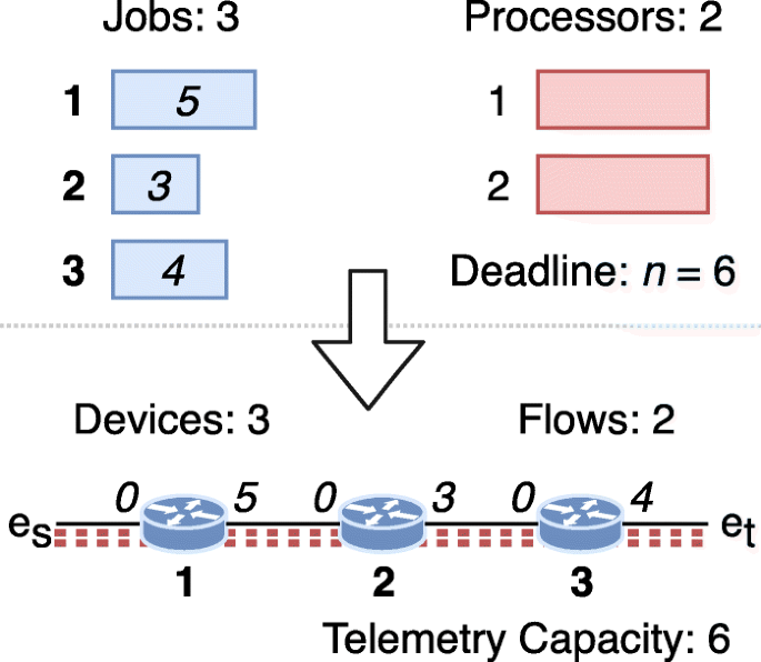

  

  Example MSP reduction to INTO Balance. An MSP instance – with |J|=3 jobs, number of processors m=2, and deadline n=6 – is reduced to an INTO Concentrate instance – with 3 forwarding devices and 2 flows with telemetry capacity equal to 6

• 2. Next, m flows P₁,P₂,...,P_m are created. Each flow has endpoints e_s and e_t and is routed through a path comprising all device interfaces in G, i.e., ρ(P_i)=(1,e_s),(1,2),(2,1),...,(|J|,e_t),i=1,2,...,m. The telemetry capacity of all flows is n.

Theorem 2

The INTO Balance decision problem is NP-Complete.

Proof

By the instance of the reduction presented, if an MSP instance has a solution schedule where all jobs finish within n time units, then the INTO Balance problem has a solution with no more than n items assigned to be transported by any single flow. Consider that each job j of length l_j scheduled to a processor P_i corresponds to the coverage of the interface of device j (with positive telemetry demand) by flow P_i. Conversely, if the INTO Balance problem has a solution where each flow is assigned to collect no more than n telemetry items, then the corresponding MSP instance has a solution where every job complete within n time units. Covering the positive demand interface of device j with flow P_i corresponds to scheduling a job of length l_j to process P_i. Lemmas 3 and 4 complete the proof. □

4 Heuristic algorithms for in-band network telemetry orchestration

In this section, we propose and formalize two heuristic algorithms (Concentrate and Balance) designed to produce high-quality solutions to the two optimization problems (INTO Concentrate and INTO Balance, respectively) in a timely manner.

4.1 Concentrate heuristic algorithm

As mentioned in Section 3.1, given the challenge of optimizing in-band telemetry orchestration, one possible strategy is to minimize the number of flows that will be used to transport telemetry data. In this section, we propose Concentrate, a heuristic algorithm focused on minimizing this number. Algorithm 1 shows the pseudo-code of Concentrate. Next, we detail its procedures.

The algorithm has two input parameters: the set I of all active device interfaces and the set F of all packet flows in the network. The algorithm maintains two main data structures, CoveredBy and Monitors, that indicate which flow covers each interface (i.e., function Φ) and which interface is to be monitored by each flow, respectively. These data structure also constitute the algorithm’s output that is used to generate packet processing rules and configure a network. Initially, no flow has been assigned to monitor any interface yet; in Lines 1-2, CoveredBy and Monitors are initialized to reflect this.

The algorithm also maintains four other auxiliary variables: κ_r (Line 3), NIFs (Line 4), SIFs (Line 5), and UFs (Line 6). Variable κ_r indicates the remaining telemetry capacity available for each flow. It is initialized with the telemetry capacity κ of the flows and is updated as assignments are made by the algorithm. NIFs indicates, for each flow, the number of interfaces not yet covered in its path. Variable SIFs keeps a sorted list of the interfaces in the path of a flow ordered non-decreasingly by the number of flows passing through them (and by the telemetry demand in case of a tie). Set UFs consists of all currently unassigned flows, initially UFs =F. Lines 7-16 contain the main repeat loop of the algorithm. At each iteration of the outermost loop, the algorithm first selects the unassigned flow f_max with the maximum number of interfaces still not covered in its path (Line 7) and removes it from UFs (Line 8). In case of a tie, the algorithm selects any of the flows with the maximum telemetry capacity. After finding f_max from F, it is assigned to monitor every interface still uncovered in its path following the ordering given by SIF(f) (Lines 10-13) and respecting its telemetry capacity (Lines 11). The remaining telemetry capacity is updated after each assignment (Line 14). For every assignment, the value of NIFs of all flows traversing the interface just covered is decreased by one (Lines 15-16), as the interface is no longer uncovered and new flows cannot be assigned to monitor it. The main loop is repeated until every flow has been considered or all interfaces have been covered by the solution.

The worst-case computational complexity of this algorithm is given by $\mathcal {O}(n) + \mathcal {O}(m) + \mathcal {O}(m \cdot n \cdot \log n) + \mathcal {O}((n + m) \cdot (n\cdot m)) = \mathcal {O}(n^{2}\cdot m + n\cdot m^{2})$, where n is the number of interfaces in I and m is the number of flows in F. Therefore, the algorithm runs in polynomial time to the number of interfaces and flows in the network.

4.2 Balance heuristic algorithm

In this subsection, we formalize the Balance algorithm, which strives to minimize the maximum number of telemetry items to be transported by any single flow. Algorithm 2 shows the pseudo-code of Balance. Balance has the same input parameters and output data structures of Algorithm 1. Algorithm 2 also maintains the same κ_r and NIFs variables of Concentrate, which indicate the remaining telemetry capacity and the number of interfaces not yet covered in the path of each flow, respectively. Balance has two additional variables: NFs and NCIFs. NFs indicates, for every interface, the number of flows with available capacity passing through it. NCIFs is the set of all intefaces that are not yet covered by any flow.

Lines 7-19 contain the main repeat loop of the algorithm. At each iteration of the outermost loop, the algorithm first selects the uncovered interface i_mm with the minimum number of flows with available capacity passing through it (Line 8) and removes it from NCIFs (Line 9). In case of a tie, any of the interfaces with maximum telemetry demand may be chosen. Next, from all flows traversing i_mm, the f_min flow collecting the least amount of telemetry items (i.e., κ(f)−κ_r(f)) out of those with available capacity is selected (Lines 10-11). In case of a tie, the flow with the minimum number of interfaces still not covered in its path is chosen. If the tie persists, the algorithm selects any one of the flows that tied in both of the steps. When i_mm and f_min have been found, flow f_min is assigned to monitor interface i_mm (Lines 12-13). After the assignment, some adjustments are made to variables κ_r, NIFs, and NFs. The remaining capacity κ_r of flow f_min is decreased by the demand δ of interface i_mm (Line 14). The number of uncovered interfaces NIFs is decreased by one for every flow passing through interface i_mm (Lines 15-16). If f_min has used all its capacity (Line 17) after been assigned to monitor i_mm, then it is necessary to update the NFs value for every interface through which f_min passes (Lines 18-19). This procedure is repeated until all active device interfaces in the network are covered, or there is not any flow with available capacity.

The worst-case complexity of this algorithm is given by $\mathcal {O}(n + m) + \mathcal {O}((n + m)\cdot (n + m)) = \mathcal {O}(n^{2} + m^{2})$, where n is the number of interfaces in I and m is the number of flows in F.

5 Evaluation

In this section, we present computational experiments with the models and algorithms introduced in the previous two sections of this paper. We start by describing the experimental setup and the dataset used in the experiments. Then, we detail two sets of experiments. The first set of experiments evaluates the proposed mathematical programming models and heuristic algorithms with regards to solution quality and processing time. We refer to the models of Section 3 as CMP (Concentrate) and BMP (Balance) and to the algorithms of Section 4 as CH (Concentrate Heuristic) and BH (Balance Heuristic). The second set of experiments compares the heuristics with regards to the performance factors introduced in Section 2. We also use the “full assignment” introduced in Section 2 as a baseline (and refer to it as FA).

The experiments were carried out in a computer with an Intel Core i7-5557U CPU running at 3.10GHz, 16GB of DDR3 1867MHz RAM, and Apple macOS 10.12 operating system. The GLPK Solver¹ 4.65 was used to solve the mathematical programs. The computation time limit to find a solution was set to 10 min. The proposed heuristic algorithms were implemented in C++ and compiled with the Apple LLVM version 9.0.0 (clang-900.0.39.2) compiler.

The dataset used in the experiments is composed of 260 topologies of real wide area networks catalogued by the Internet Topology Zoo (ITZ) project [20] and traffic matrices made available in Repetita [21]. ITZ topologies range from 4 to 197 points-of-presence and from 16 to 880 interfaces. The maximum (minimum) network diameter is 37 (3) hops. To generate realistic traffic matrices, Gay et al. [21] followed the randomized gravity model proposed in [22]. We converted the available topologies to INTO problem instances. For every link in the topology, we considered there were two interfaces, one in each extremity. Interface telemetry demands were randomly chosen from the range from four to ten items following a uniform distribution. We choose this range since four can be considered the minimum amount of items to identify the source of a metadata field and its value (e.g., device ID + queue ID + queue ingress timestamp + queue delay) and ten is the number of common metadata fields that can be exported by devices according to [23]. For each pair of network endpoints with positive demands according to the traffic matrices, we considered there is a single aggregate network flow (i.e., we differentiate flows by the pair of network entry point and exit point). Flow telemetry capacities were randomly chosen following a normal distribution. Otherwise stated, the mean telemetry capacity is equal to 35 items, and the standard deviation is 5 items, which amounts for approximately 10% of the MTU being available for transporting metadata in each packet.

5.1 Mathematical programming models and heuristic algorithms

To work in practice, a procedure to solve any variation of the INTO problem should be able to provide high-quality solutions within short time intervals. This is necessary so that the monitoring campaign can quickly adapt to network policy changes and traffic fluctuation. In this first set of experiments, we evaluate the solution quality and processing time of the algorithms introduced in Section 4, namely Concentrate Heuristic (CH) and Balance Heuristic (BH), by comparing them to the mathematical programming models.

We start by analyzing the processing times of the approaches. Figure 6 shows the time taken by the GLPK Solver to run each of the INTO problem instances for the mathematical programming models. As expected, it grows quickly with relation to instance size for both models. We note that the time to process an instance is also subject to other network characteristics besides size (e.g., diameter, degree of connectivity of nodes, heterogeneity of paths). Thus, in the graphs, we can expect that some networks, although smaller than other, take more time to be solved.

Fig. 6

Processing times for the mathematical programming models

For the Concentrate Mathematical Program (CMP) model, the solver was not able to find an optimal solution and check optimality for networks with more than 90 interfaces (14 devices) within the 10-min time limit. The solver was able to find the optimal solution within the time limit for the INTO Balance instances with up to 252 interfaces (56 devices) using the Balance Mathematical Program (BMP) model. From these results, we conclude that solving CMP is generally harder than BMP. The difference in processing time between the two approaches can be attributed in part to the fact that the mathematical model CMP has more decision variables than BMP. Models with more variables tend to have larger solution spaces and, thus, take longer to explore their totality in order to check optimality. In summary, Fig. 6 shows that solving both versions of the INTO problem using the mathematical models takes considerable time, making their use impracticable in real, highly dynamic scenarios.

Figure 7 shows the processing time of the heuristic algorithms CH and BH as a function of the network size. Both algorithms generate feasible solutions to all instances of their corresponding INTO variation in less than one second. These results are up to three orders of magnitude lower than the processing times required by the mathematical models. The short processing times achieved by both heuristic algorithms argues in favor of their adequacy to be applied in highly dynamic networks. Next, to confirm that they are adequate, we also evaluate the quality of the solutions given by them.

Fig. 7

Processing times for the heuristic algorithms.

To evaluate the quality of the solutions provided by the heuristics, we compare their objective function values to lower bound models. We start by comparing the lower bound models and the mathematical programming models to estimate how close to the optimal values are the lower bounds. Then, we compare the lower bounds with the heuristic algorithms solutions considering the estimated gap. The lower bound for INTO Concentrate is computed by exchanging Eq. 3 of the CMP model by Eq. 12². The original equation had two purposes: (i) guarantee that no flow is assigned to collect and transport more items then its capacity allows and (ii) activate the variable y_f (which is used by the objective function of CMP to count the number of telemetry-active flows) when any telemetry item is assigned to flow f∈F. With the new equation we assume a scenario where all flows would have unlimited telemetry capacity. The new, simpler constraint presented in Eq. 12 does not consider telemetry demands and capacities (first purpose), eliminating a summation and making it quicker to compute. Only the second purpose of the original equation is kept, i.e., all flows performing at least one telemetry action will be accounted for in the objective function.

$$ x_{i,f} \leq y_{f}, \forall i \in I, \forall f \in F $$

(12)

In our experiments, the solver was able to find feasible solutions for the CMP model for 248 out of the 260 networks. Out of those 248 cases, the solver was able to certify optimality for only 28 instances. No feasible solution was found for 12 problem instances. The mean gap between the lower bound and CMP across all 248 feasible solutions found by the solver was 12.62 flows (with standard deviation equal to 11.68 flows). The minimum and maximum gap values were 0 and 50 flows, respectively. Compared to the lower bound, the mean gap for CH was 9.82, and the standard deviation was 7.93. The minimum and maximum gap values were 0 and 49 flows. Comparing the gaps, we conclude that the solutions generated by CH are slightly better than the feasible solutions provided by the CMP model within the 10-min time limit. Thus, the CH algorithm is not only able to generate solutions within one second but also provides high-quality solutions.

To evaluate the quality of the solutions found to the INTO Balance variation, we compute a lower bound for each instance as the maximum value between (i) the maximum telemetry demand of a single interface and (ii) the sum of all demands divided by the total number of flows.

Out of all 260 instances evaluated, for the BMP model, the solver was able to find feasible solutions within the time limit for 223. The solver was able to certify optimality for 174 out of these 223 cases. No feasible solution was found within 10 min for 37 instances. In our comparison, the optimal solution matched the lower bound in 171 out of the 174 optimal cases. Considering all 223 feasible solutions found, the mean lower bound to BMP gap was 0.84 items (with standard deviation equal to 2.37). The minimum and maximum gap values were 0 and 14 items, respectively. Concerning the BH algorithm, the mean gap to the INTO Balance lower bound was 0.09 items (the standard deviation was 0.63). The minimum and maximum gap values were 0 and 5 items. The BH algorithm was able to generate an optimal solution for all but 5 instances. Both BMP and BH have solutions with object function values very close to the lower bounds.

From the experiments in this subsection we conclude that both of the proposed algorithms, CH and BH, generate high-quality solutions within short processing times, and, thus, are well suited to be applied in highly dynamic networks.

5.2 Comparison of the INTO problem variations

When optimizing the use of INT to perform monitoring, an operator may opt to configure the network according to one of the two variations of the INTO problem. In this remaining set of experiments, we compare the solutions generated by the proposed heuristic algorithms (CH and BH) and the baseline full assignment (FA) introduced in Section 2. To evaluate the algorithms, we consider the main INT constraints and performance influencing factors discussed in Section 2.

5.2.1 Maximizing interface coverage

As previously discussed in Section 2, the telemetry capacity of flow packets in a network may limit how many of the device interfaces can be monitored. In this subsection, we evaluate how sensitive the INT orchestration strategies are regarding interface coverage.

For each of the assignment strategies, we set the initial mean packet telemetry capacity to 5 items (the standard deviation was kept at 5 items for the whole experiment). We then calculated the interface coverage – i.e., the percentage of device interfaces covered by at least one flow – for every network of the Internet Topology Zoo [20]. Finally, we increase the mean capacity in steps of 5 items until each assignment strategy was able to provide a solution with full (100%) coverage for all networks. Fig. 8 presents the results of this experiment as a CDF where the x-axis indicates coverage levels and the y-axis indicates percentages of the networks. For every pair of strategy and capacity level, we plot a curve in the graph. For the full assignment (FA curves in the plot), we report the real coverage levels that would be achieved without exceeding the packet MTU (i.e., telemetry capacity).

Fig. 8

Interface Coverage

The main conclusion from the results presented in Fig. 8 is that the proposed heuristics (CH and BH) are more resilient to lower levels of telemetry capacity than the full assignment (FA). Even when the capacity is at its lowest level (5 items), they can achieve 100% interface coverage (full coverage) for about 25% of the networks. Furthermore, in the same scenario, about 80% of the networks have good coverage of at least 90% of interfaces. CH and BH present similar coverage for all capacity levels, with a slightly better, yet noticeable result observed for the latter. While both of the heuristics achieve full coverage when the mean telemetry capacity is 20 items, the full assignment only achieve it when that capacity is at least 35 items.

In the following subsections, to avoid biasing or tainting the comparison, we will only present and consider the results where each strategy was able to achieve full coverage for all networks. That is, when the capacity is of at least 35 and 20 items for the full assignment and heurstic algorithms, respectively. Next, we continue the evaluation by considering quality and cost metrics related to the four performance factors introduced in Section 2.

5.2.2 Minimizing flow packet load

As introduced in Section 2 (Item (a)), one of the INT factors that may influence network performance is intrinsically related to the extent to which packets vary in size along their paths. The number of telemetry items flow packets collect from device interfaces (i.e., its telemetry load) determines this variation. The best approach to avoid causing significant jitter or drift in transmission times is to minimize the telemetry load of packets. Fig. 9 presents the cumulative distribution function of the mean flow packet load. For each orchestration strategy, the figure presents a curve representing the distribution of values when the mean telemetry capacity ($\bar {\kappa }$) is 35 items. The figure also presents 95% confidence intervals as filled areas in the graph.

Fig. 9

Mean and confidence interval for flow packet load when the mean telemetry capacity is 35 items

The results in Fig. 9 show that BH achieves the best possible telemetry load per flow packet. The mean load is approximately seven items, which is also the mean telemetry demand of interfaces. This value indicates that in its solutions, BH tends to assign each telemetry-active flow to monitor one interface. The variability shown in the graph for BH is due to the variation of the interface telemetry demands. In all cases, CH and FA present higher load values than BH. CH presents higher values than BH because when minimizing the number of telemetry-active flows it tends to use as much as possible the capacity of (a small subset of) flows. CH also presents high variability for flow packet load, which is due to its greedy rationale to flow assignment. Its heuristic causes a group of flows to use most of their packet capacity while another group uses only a fraction to cover the remaining interfaces.

Figure 10 illustrates the influence of the mean capacity of flow packets over the mean telemetry load. It reveals that BH is not influenced by the capacity. This phenomenon was expected since an increase in capacity has no impact in minimizing the maximum flow packet load (i.e., the optimization goal of BH). CH presents small increases in flow load as capacity increases. In turn, FA increases significantly the telemetry load imposed on flows when more capacity is available, which aligns with its objective of collecting as many items as possible with all flows. In a case where the telemetry capacity is assumed to be infinite, the mean flow packet load of FA would be an approximation of the mean telemetry demand of all flow paths in a network.

Fig. 10

Evaluation of flow load as telemetry capacity varies

5.2.3 Minimizing flow usage

The limitation on the processing capacity of forwarding devices and monitoring sinks (Section 2, Items (b) and (c)) prompts orchestration strategies to minimize the number of telemetry reports generated periodically. This minimization has the objective of alleviating the packet processing overhead on both forwarding devices and monitoring sinks/analyzers. In this subsection, we evaluate the flow usage (i.e., the number of telemetry-active flows) demanded by the strategies, as this number directly influences the number of reports generated.

Figure 11 presents the flow usage as a function of the number of device interfaces in a network. For every combination of strategy, telemetry capacity and network we plot a point in the graph. We limit the y-axis to 1 800 flows to be able to compare the flow usage of the proposed heuristics. The total number of flows for the largest tested network (i.e., the one with 880 interfaces) is 38 612.

Fig. 11

Flow usage as a function of the number of interfaces in a network

CH uses the minimum amount of flows across all strategies, which was expected since its main optimization objective is to minimize this value. CH typically assigns each telemetry-active flow to monitor about four interfaces, a 4:1 interface to flow ratio. BH presents a direct relationship between the number of active flows and of interfaces, i.e., each flow covers a single interface (1:1 ratio). Thus, BH uses, in the general case, four times more flows than CH. For a mean telemetry capacity of 35 items, CH uses 225 flows to cover the largest network in the dataset, which has 880 forwarding device interfaces, while BH uses 880 flows. For the same scenario, FA assigns all 38 612 flows (not shown in the graph) in the network to carry out telemetry. Thus, both of the heuristics use up to two orders of magnitude less flows then FA. CH is the most scalable of the strategies, followed by BH with a multiplicative increase by a constant factor of about four.

5.2.4 Maximizing information correlation

In addition to minimizing the number of telemetry-active flows, the limited processing capacity of monitoring sinks (Section 2, Item (c)) also motivates strategies to maximize the correlation of the information contained in each telemetry report received by the monitoring sinks, simplifying their analysis. In this evaluation, we consider the percentage of interfaces a flow covers from its path as a measure of this correlation.

The results of the experiment are shown in Figs. 12 and 13. Figure 12 presents the CDF of the mean information correlation for the networks. The graph has a curve for each evaluated strategy showing the distribution of values when the mean telemetry capacity is 35 items. The figure also presents the 95% confidence intervals as filled areas in the graph. Figure 13 shows the effect of the telemetry capacity on the mean correlation. For clarity, we omit confidence intervals in this second figure.

Fig. 12

Mean and confidence interval for information correlation when the mean telemetry capacity is 35 items

Fig. 13

Evaluation of information correlation as the telemetry capacity of flows varies

The results in Figs. 12 and 13 support the expected behavior of the heuristics. According to Fig 12 CH presents the best results among the heuristics, with (the top) da85% of networks having 50% or more information correlation. Note in the figure that the lower 15% of the networks (0%–15%) have an x-axis value below 50, while the remaining 85% (15%–100%) have a value equal or above 50. This means that a typical report covers at least half the path of a flow. We highlight that the results for FA in Fig. 13 show that reaching high correlation is very costly in terms of packet telemetry capacity. More specifically, to achieve 90% correlation for about 85% of the networks, the mean telemetry capacity must be about 50 items per packet. Observe (in Fig. 13) that the lower 15% of the networks have an x-axis value below 90 for curve FA ($\bar {\kappa } = 50$), while the remaining upper 85% have values above 90.

Going back to Fig. 12, it also presents the significant variability in flow assignment (see filled area) regarding CH found previously in Fig. 9. This behavior confirms the previous conclusion that CH tends to assign a group of flows to cover (almost) their entire path, while another group covers only a few remaining interfaces each. BH is not influenced by telemetry capacity variation. This is concluded by the fact that all curves for BH in Fig. 13, representing different levels of telemetry capacity, superimpose each other. BH achieves at least 25% correlation for most of the networks in all scenarios, i.e., flows tend to cover about one-fourth of their paths.

5.2.5 Optimizing information freshness

As the last aspect of our comparison, the limitation on link bandwidth (Section 2, Item (d)) argues for (i) avoiding transporting telemetry data through too many links in a network and for (ii) distributing the origin of telemetry reports as much as possible among network devices. The mean information freshness – i.e., the mean number of hops the information collected at interfaces is transported in-band before being reported to a monitor sink – enables us to measure to which extent the strategies conform to this task.

Figs. 14 and 15 present the freshness results. Figure 14 shows the CDF of the mean information freshness considering the three orchestration strategies. The filled areas in the graph represent the 95% confidence intervals. Figure 15 shows the freshness as a function of the network diameter (i.e., the length of the longest flow path).

Fig. 14

Mean and confidence interval for information freshness with mean telemetry capacity equal to 35 items

Fig. 15

Information freshness as a function of the network diameter

BH keeps information freshness at the optimal value (zero) for most of the networks analyzed (Fig. 14). A value zero for freshness indicates that most information is reported to a monitoring sink immediately after being collected, which results in the best possible monitoring traffic distribution across a network. Figure 15 indicates that the network diameter has little to no effect on freshness for BH. FA typically causes flows to transport telemetry information for about two hops before reporting it. The freshness has slightly worse values for larger networks. CH presents the worst freshness values among strategies and is significantly influenced by the network diameter. CH comes to the point of making flows transport information up to 10 hops (in the mean case) for networks with a diameter of about 33 hops. Thus, CH tends to concentrate more the points where reports are generated, which may lead to link saturation.

6 Related work

In this section, we review previous work that investigated the use of network and device mechanisms to monitor networks and services.

NetSight [2] has packet mirroring as its fundamental monitoring piece, which is available in both OpenFlow [24] and traditional switches. In NetSight, every switch in the path of a packet creates a copy of it, called postcard, and sends it to a logically centralized control plane. The multiple postcards of a single packet passing through the network are combined in the control plane to form a packet history that tells the complete path the packet took inside the network and the modifications it underwent along the way. Depending on the size and level of activity of the network, NetSight may generate a considerable volume of monitoring data. To overcome this issue, Everflow [3] applies a match+action mechanism to filter packets and decide which ones should be mirrored, thus reducing the overheads at the cost of monitoring accuracy and level of detail. Stroboscope [4] also applies packet mirroring to monitor networks. It answers monitoring queries by scheduling the mirroring of millisecond-long slices of traffic while considering a budget to avoid network performance degradation.

Payless [5] and AdaptiveSampling [6] followed a different direction of the previous work. They make use of two OpenFlow-enabled switch features to monitor a network: (i) the capability to store statistics related to table entries (which may represent flows) and (ii) the possibility of exporting these statistics via a polling mechanism. In these works, the polling frequency influences the quality (e.g., freshness) of the monitoring data. The higher the frequency, the more fine-grained the data. Payless and AdaptiveSampling dynamically and autonomously adjust the polling frequency to achieve a good trade-off between monitoring quality and cost. Another work in the context of software-defined measurement is DREAM [25]. DREAM is a system that dynamically adapts resources (i.e., TCAM entries) allocated to measurement tasks and partitions each of them among devices. DREAM supports multiple concurrent tasks and ensures that estimated values meet operator-specified levels of accuracy. Payless, AdaptiveSampling and DREAM have the goal of monitoring traffic characteristics and keeping costs low. Assessing the network state (e.g., switch queue occupancy) is outside their scope.

The idea of orchestrating monitoring data collection across multiple devices to reduce costs is not new. Several investigations have been carried out with that objective. For example, Cormode et al. [26] proposed configuring devices to independently monitor their local variables and only report their values (to a centralized coordinator) when significant changes are observed. A-GAP [27] and H-GAP [28] organize measurement nodes into a logical tree graph. When a significant change is observed for a local variable, the node sends an update to its parent node. The latter node is responsible for aggregating the values from multiple devices and sending updates up the tree upon significant value change. The root node maintains network-wide aggregate values to be used for monitoring analysis. Tangari et al. [29] proposed decentralizing monitoring control. The monitoring control plane is composed of multiple distributed modules, each capable of performing measurement tasks independently. Their approach logically divides the network into multiple monitoring contexts, each with specific requirements. As a result, monitoring data tends to be aggregated and analyzed close to the source, reducing considerably the communication overhead. The rationale behind these works was conceived before the emergence of programmable data planes without considering the opportunity to programming it. As a consequence, in contrast to INTO, their solutions are based on traditional coarse-grained counters and aggregate statistics and their data exchange models operate at control plane timescales.

More recently, with the emergence of programmable data planes and P4 [8], several works have explored programming forwarding devices to carry out custom, monitoring-oriented packet processing. For example, HashPipe [30] is an algorithm that implements a custom pipeline targeting programmable data planes [7, 31, 32] to detect heavy hitters. Snappy [33] and NCDA [34] focus on the use of in-switch memory and the visibility into device queue occupancy provided by P4 to detect congestion events, identify the offending flows, and execute congestion avoidance actions. These works contrast with ours in that they are focused on device-wise monitoring tasks, while INTO orchestrates network-wide monitoring telemetry.

A work more related to our context is Sonata [35], a system that coordinates the collection and analysis of network traffic to answer operator-defined monitoring queries. These queries consist of a sequence of dataflow operators (e.g., filter, map, reduce) to be executed over a stream of packets. Sonata is based upon stream processing systems and programmable forwarding devices, partitioning queries across them. Similar to INTO, it has the goal of minimizing the amount of data that needs to be sent to and analyzed by the control plane (i.e., stream processors). Sonata leverages data plane programmability to offload as much as possible of each query to the forwarding devices, considerably reducing the packet stream before sending it to stream processors. Different from INTO – which targets monitoring network state, behavior and performance – Sonata focuses on the analysis of traffic characteristics. Furthermore, Sonata does not apply in-band network telemetry for metadata reporting.

In our work, we revisit the challenge of monitoring networks effectively and efficiently. We identify the new opportunities for obtaining accurate and fine-grained information about forwarding device state, behavior and performance considering the recent advances in SDN and programmable networks. In a previous work [15], we have taken an initial step towards understanding the trade-offs involved in conducting network monitoring via a mechanism such as in-band network telemetry (INT) [10–12]. We identified the key factors that impact performance associated with it and proposed heuristic algorithms to orchestrate INT tasks to minimize overheads. In the current paper, we build upon our previous work [15] by formalizing in-band network telemetry orchestration as an optimization problem. We also prove that it is an NP-Complete problem, proposing integer linear programming models to solve it. And, finally, redesign the proposed heuristics to both better suit realistic network scenarios and produce high-quality solutions within strict computational time.

7 Conclusion

This work introduced the In-band Network Telemetry Orchestration (INTO) problem. It consists in minimizing monitoring overheads in the data, control and management planes when using In-band Network Telemetry (INT) to collect the state and behavior of forwarding device interfaces. We formalized two variations of the INTO problem and proposed integer linear programming models to solve them. The first variation of the problem, INTO Concentrate, has the goal of minimizing the number of flows used for telemetry. The second variation, INTO Balance, seeks to minimize the maximum telemetry load (i.e., the number of telemetry items transported) among packets of distinct flows. We proved that both variations belong to the NP-Complete class of computational problems.

Through our evaluation using real networks topologies, we found that both of the proposed models take a long time to solve the INTO problem. This result motivated us to design two heuristic algorithms to produce feasible solutions in polynomial computational time to the network size and number of flows. Experimental results show that the proposed heuristics produce high-quality solutions in under 1 second for all of the real networks evaluated.

To assess the benefits and limitations of the proposed heuristics, we compared them against each other and with the baseline full assignment approach. We concluded that the heuristic to solve INTO Concentrate (CH) performs well in minimizing the overhead on forwarding devices and monitoring sinks. The number of telemetry reports that have to be generated periodically is minimal, and the information reported to sinks has a significant level of correlation to ease their analysis. As a consequence, CH is the most scalable of the strategies and may be particularly recommended for medium to large networks. The INTO Balance heuristic (BH) imposes the lowest telemetry load per monitoring-active flow, and results in the best distribution of the telemetry load among forwarding devices and links in a network. These results suggest that BH may be an adequate strategy for low latency networks or when monitoring traffic highly sensitive to packet size changes. Both of the heuristics also scale well with network size, which contrasts to the full assignment, as it causes considerable overhead on network traffic and devices.

As future work, we intend to explore other assignment function options (e.g., interface demand partitioning, limited coverage redundancy). We also intend to investigate how to translate high-level monitoring policies to individual device interface-level demands. Finally, we plan to explore how in-band network telemetry orchestration can be used to help with tasks such as congestion avoidance and load balancing.

References

da Costa Filho RIT, Luizelli MC, Vega MT, van der Hooft J, Petrangeli S, Wauters T, De Turck F, Gaspary LP. Predicting the performance of virtual reality video streaming in mobile networks. In: Proceedings of the 9th ACM Multimedia Systems Conference, MMSys’18. New York: ACM: 2018. p. 270–83. http://doi.acm.org/10.1145/3204949.3204966.
Handigol N, Heller B, Jeyakumar V, Mazieres D, McKeown N. I know what your packet did last hop: Using packet histories to troubleshoot networks. In: Proceedings of the USENIX Conference on Networked Systems Design and Implementation, NSDI’14. Berkeley: USENIX Association: 2014. p. 71–85. http://dl.acm.org/citation.cfm?id=2616448.2616456.
Zhu Y, Kang N, Cao J, Greenberg A, Lu G, Mahajan R, Maltz D, Yuan L, Zhang M, Zhao BY, Zheng H. Packet-level telemetry in large datacenter networks. In: Proceedings of the ACM SIGCOMM Conference, SIGCOMM ’15. New York: ACM: 2015. p. 479–91. http://doi.acm.org/10.1145/2785956.2787483.
Tilmans O, Bühler T, Poese I, Vissicchio S, Vanbever L. Stroboscope: Declarative network monitoring on a budget. Renton: USENIX NSDI; 2018.
Chowdhury SR, Bari MF, Ahmed R, Boutaba R. Payless: A low cost network monitoring framework for software defined networks. In: Proceedings of the IEEE Network Operations and Management Symposium, NOMS’14: 2014. p. 1–9. http://doi.org/10.1109/NOMS.2014.6838227.
Cheng G, Yu J. Adaptive sampling for openflow network measurement methods. New York: ACM; 2017. pp. 4:1–4:7. http://doi.acm.org/10.1145/3095786.3095790.
Bosshart P, Gibb G, Kim HS, Varghese G, McKeown N, Izzard M, Mujica F, Horowitz M. Forwarding metamorphosis: Fast programmable match-action processing in hardware for sdn. In: Proceedings of the ACM SIGCOMM Conference, SIGCOMM ’13. New York: ACM: 2013. p. 99–110. http://doi.acm.org/10.1145/2486001.2486011.
Bosshart P, Daly D, Gibb G, Izzard M, McKeown N, Rexford J, Schlesinger C, Talayco D, Vahdat A, Varghese G, Walker D. P4: Programming protocol-independent packet processors. SIGCOMM Comput Commun Rev. 2014; 44(3):87–95. http://doi.acm.org/10.1145/2656877.2656890.
Chole S, Fingerhut A, Ma S, Sivaraman A, Vargaftik S, Berger A, Mendelson G, Alizadeh M, Chuang ST, Keslassy I, Orda A, Edsall T. drmt: Disaggregated programmable switching. In: Proceedings of the Conference of the ACM Special Interest Group on Data Communication, SIGCOMM ’17. New York: ACM: 2017. p. 1–14. http://doi.acm.org/10.1145/3098822.3098823.
Jeyakumar V, Alizadeh M, Geng Y, Kim C, Mazières D. Millions of little minions: Using packets for low latency network programming and visibility. SIGCOMM Comput Commun Rev. 2014; 44(4):3–14. http://doi.acm.org/10.1145/2740070.2626292.
Kim C, Sivaraman A, Katta N, Bas A, Dixit A, Wobker LJ. In-band network telemetry via programmable dataplanes. In: Posters and Demos of the ACM SIGCOMM Symposium on SDN Research, SOSR’15. Santa Clara: 2015. http://git.io/sosr15-int-demo.
Thomas J, Laupkhov P. Tracking packets’ paths and latency via int (in-band network telemetry) 3rd P4 Workshop (2016). https://2016p4workshop.sched.com/event/6otq/using-int-to-build-a-real-time-network-monitoring-system-scale.
Ozdag R. Intel® Ethernet Switch FM6000 Series-Software Defined Networking. 2012. Tech. rep., Intel Corporation. https://people.ucsc.edu/~warner/Bufs/ethernet-switch-fm6000-sdn-paper.pdf.
Zhang Q, Liu V, Zeng H, Krishnamurthy A. High-resolution measurement of data center microbursts. In: Proceedings of the Internet Measurement Conference, IMC ’17. New York: ACM: 2017. p. 78–85. http://doi.acm.org/10.1145/3131365.3131375.
Marques JA, Gaspary LP. Explorando estratégias de orquestração de telemetria em planos de dados programáveis. Anais do Simpósio Brasileiro de Redes de Computadores e Sistemas Distribuídos (SBRC). 2018; 36.
Cordeiro WLdC, Marques JA, Gaspary LP. Data plane programmability beyond openflow: Opportunities and challenges for network and service operations and management. J Netw Syst Manag. 2017; 25(4):784–818. https://doi.org/10.1007/s10922-017-9423-2.
Lee M, Duffield N, Kompella RR. Not all microseconds are equal: Fine-grained per-flow measurements with reference latency interpolation. In: Proceedings of the ACM SIGCOMM 2010 Conference, SIGCOMM ’10. New York: ACM: 2010. p. 27–38. http://doi.acm.org/10.1145/1851182.1851188.
Quinn P, Elzur U, Pignataro C. Network Service Header (NSH) RFC 8300. Internet Engineering Task Force (IETF) (2018). https://tools.ietf.org/html/rfc8300.
Garey MR, Johnson DS. Computers and Intractability: A Guide to the Theory of NP-Completeness. New York: W. H. Freeman & Co.; 1979.
Knight S, Nguyen HX, Falkner N, Bowden R, Roughan M. The internet topology zoo. IEEE J Sel Areas Commun. 2011; 29(9):1765–75. https://doi.org/10.1109/JSAC.2011.111002.
Gay S, Schaus P, Vissicchio S. REPETITA: Repeatable Experiments for Performance Evaluation of Traffic-Engineering Algorithms. 2017. https://arxiv.org/abs/1710.08665.
Roughan M. Simplifying the synthesis of internet traffic matrices. SIGCOMM Comput Commun Rev. 2005; 35(5):93–6. http://doi.acm.org/10.1145/1096536.1096551.
The P4.org Applications Working Group. In-band Network Telemetry (INT) dataplane specification: P4.org; 2018. https://github.com/p4lang/p4-applications/blob/master/docs/INT.pdf.
McKeown N, Anderson T, Balakrishnan H, Parulkar G, Peterson L, Rexford J, Shenker S, Turner J. Openflow: Enabling innovation in campus networks. SIGCOMM Comput Commun Rev. 2008; 38(2):69–74. http://doi.acm.org/10.1145/1355734.1355746.
Moshref M, Yu M, Govindan R, Vahdat A. Dream: Dynamic resource allocation for software-defined measurement. In: Proceedings of the 2014 ACM Conference on SIGCOMM, SIGCOMM ’14. New York: ACM: 2014. p. 419–30. http://doi.acm.org/10.1145/2619239.2626291.
Cormode G, Garofalakis M, Muthukrishnan S, Rastogi R. Holistic aggregates in a networked world: Distributed tracking of approximate quantiles. In: Proceedings of the 2005 ACM SIGMOD International Conference on Management of Data, SIGMOD ’05. New York: ACM: 2005. p. 25–36. http://doi.acm.org/10.1145/1066157.1066161.
Prieto AG, Stadler R. A-gap: An adaptive protocol for continuous network monitoring with accuracy objectives. IEEE Trans Netw Serv Manag. 2007; 4(1):2–12. https://doi.org/10.1109/TNSM.2007.030101.
Jurca D, Stadler R. H-gap: estimating histograms of local variables with accuracy objectives for distributed real-time monitoring. IEEE Trans Netw Service Manag. 2010; 7(2):83–95. https://doi.org/10.1109/TNSM.2010.06.I8P0292.
Tangari G, Tuncer D, Charalambides M, Pavlou G. Decentralized monitoring for large-scale software-defined networks. In: Proceedings of the IFIP/IEEE Symposium on Integrated Network and Service Management (IM): 2017. p. 289–97. https://doi.org/10.23919/INM.2017.7987291.
Sivaraman V, Narayana S, Rottenstreich O, Muthukrishnan S, Rexford J. Heavy-hitter detection entirely in the data plane. In: Proceedings of the Symposium on SDN Research, SOSR ’17, pp. 164–176. ACM, New York, NY, USA (2017). http://doi.acm.org/10.1145/3050220.3063772.
Barefoot. Barefoot Tofino™. https://barefootnetworks.com/products/brief-tofino/. Acessed on May, 14 2019.
Cavium. XPliant® Ethernet Switch Product Family. https://www.cavium.com/xpliant-ethernet-switch-product-family.html. Accessed on May, 14 2019.
Chen X, Feibish SL, Koral Y, Rexford J, Rottenstreich O. Catching the microburst culprits with snappy. In: Proceedings of the Afternoon Workshop on Self-Driving Networks SelfDN 2018. New York: ACM: 2018. p. 22–8. http://doi.acm.org/10.1145/3229584.3229586.
Turkovic B, Kuipers F, van Adrichem N, Langendoen K. Fast network congestion detection and avoidance using p4. In: Proceedings of the 2018 Workshop on Networking for Emerging Applications and Technologies, NEAT ’18. New York: ACM: 2018. p. 45–51. http://doi.acm.org/10.1145/3229574.3229581.
Gupta A, Harrison R, Canini M, Feamster N, Rexford J, Willinger W. Sonata: Query-driven streaming network telemetry. In: Proceedings of the 2018 Conference of the ACM Special Interest Group on Data Communication, SIGCOMM ’18. New York: ACM: 2018. p. 357–71. http://doi.acm.org/10.1145/3230543.3230555.
Acknowledgements
Not applicable.
Funding
This work was partially funded by the Conselho Nacional de Desenvolvimento Científico e Tecnológico – Brasil (CNPq) project number 441892/2016-7, Coordenação de Aperfeiçoamento de Pessoal de Nível Superior – Brasil (CAPES) finance code 001, and the Rede Nacional de Ensino e Pesquisa – Brasil (RNP).
Author information
Authors and Affiliations
Contributions
JM collaborated in the formalization of the INTO problem, participated in the proposal of optimization models, participated in the formulation of the proofs of NP-completeness, participated in the design of the heuristic algorithms, coded proof-of-concept implementations, ran evaluation experiments, and participated in the analysis of results obtained from experimental evaluations. ML collaborated in the formalization of the INTO problem, participated in the proposal of optimization problems, and participated in the formulation of the proofs of NP-completeness. RT collaborated in the formalization of the INTO problem, and participated in the analysis of results obtained from experimental evaluations. LG collaborated in the formalization of the INTO problem, participated in the design of the heuristic algorithms, and analyzed results obtained from experimental evaluations. All authors wrote, read, and approved the final manuscript.
Corresponding author
Ethics declarations
Competing interests
The authors declare that they have no competing interests.
Additional information
Publisher’s Note
Springer Nature remains neutral with regard to jurisdictional claims in published maps and institutional affiliations.
Rights and permissions
Open Access This article is distributed under the terms of the Creative Commons Attribution 4.0 International License (http://creativecommons.org/licenses/by/4.0/), which permits unrestricted use, distribution, and reproduction in any medium, provided you give appropriate credit to the original author(s) and the source, provide a link to the Creative Commons license, and indicate if changes were made.
About this article
Cite this article
Marques, J., Luizelli, M., Tavares da Costa Filho, R. et al. An optimization-based approach for efficient network monitoring using in-band network telemetry. J Internet Serv Appl 10, 12 (2019). https://doi.org/10.1186/s13174-019-0112-0
Received:
Accepted:
Published:
DOI: https://doi.org/10.1186/s13174-019-0112-0